From Admission to Discharge

Dynamically Updating Length of Stay Forecasts with Causal Diagnostic and Operational Penalties

Mustafa Aslan, Cardiff University, UK
Lead supervisor: Prof. Bahman Rostami-Tabar
Co-supervisor: Dr. Jeremy Dixon
Data Lab for Social Good, Cardiff University, UK

11 June 2026

Outline

• The Operational Problem
• Solution
• The Framework
• The Causal Location Shift Example
• Counterfactual Simulation & Impact

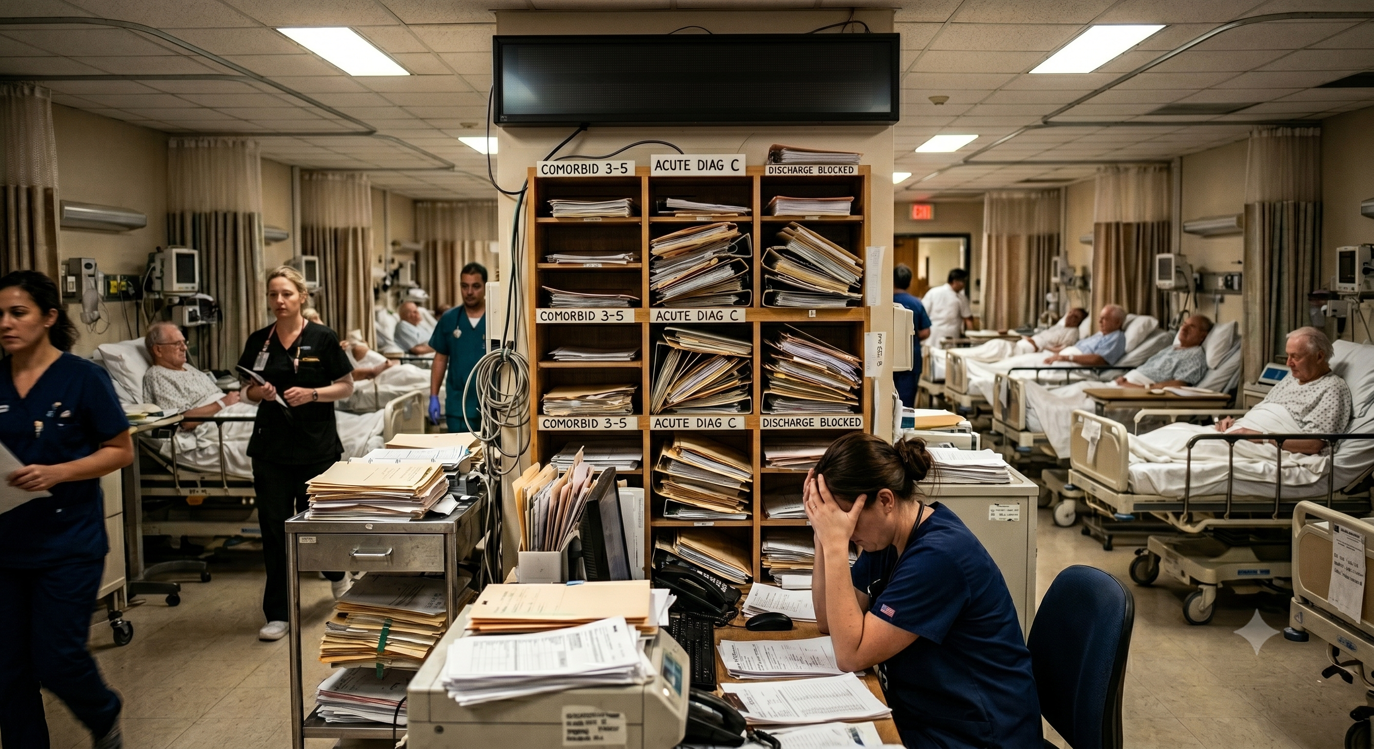
The “Operational Problem”

Current hospital operations rely on aggregate comorbidity scores (e.g., Charlson), which compress complex medical histories, masking the true operational drivers of discharge delays.

• The Problem: We cannot manage what we do not isolate.
• The Gap: Traditional models suffer from selection bias; diagnostics are endogenous.
• Our Approach: Move from “Correlative Scores” to “Causal Penalties.”

Solution

Dynamic Thresholding: Real-Time Updating

We update the survival curve (\(P(LoS > threshold)\)) dynamically as clinical data arrives (11 am daily).

1. Admission Day

• Baseline prediction based on initial exisitng data
• Initial \(P(LoS > \text{threshold})\)

➔

2. Mid-Stay Update

• Diagnosis confirmed
• Causal Shift: Apply \(\tau_D\) penalty to the distribution

➔

3. Action Trigger

• Condition: \(P(LoS > \text{threshold}) \ge 55\%\)
• Action: Refer to MDT / Community pathways

The Framework

1. Purging Confounders

We utilize Double Machine Learning (DML) to isolate the causal impact of diagnostics (\(\tau_D\)) and ward transfers (\(\tau_W\)) from the “clean-path” LoS.

\[ Y_{purged} = Total\_LoS - \sum_{i=1}^{n} \tau_{D_i} - \tau_{W_j} \]

• Identification: DML partials out high-dimensional confounders (age, gender, ward busyness) to estimate the true “bed-day burden” of specific diagnoses.

• Purging: We subtract realized shocks from the observed outcome to create an idealized survival curve \(S_0(t)\)—the “clean-path” prediction in the absence of operational friction.

The Framework

2. Modeling Uncertainty of the Diagnostic Penalty For Updating the \(\hat{LoS}\)

We treat diagnostic impact not as a fixed constant, but as a distribution, accounting for clinical uncertainty.

The Convolution

To generate a robust “Tail Risk” LoS forecasts, we convolve the baseline LoS distribution (\(f_L\)) with the diagnostic uncertainty (\(\tau_D \sim \mathcal{N}(\mu, \sigma^2)\)):

\[ f_{new}(z) = \int_{-\infty}^{\infty} f_L(z - \tau) \cdot f_\tau(\tau) \, d\tau \]

• \(f_L(z - \tau)\): The baseline LoS probability.
• \(f_\tau(\tau)\): The clinical uncertainty of the diagnostic penalty.

Why this matters for the MDT:

• Beyond the Average: It captures the “Tail Risk”—the patients who face both a complex diagnosis and a slow recovery.
• Operational Buffer: By modeling the variance of the effect (\(\sigma^2\)), we create a “safety margin” for discharge planning.
• Robustness: This prevents underestimating the probability of a patient becoming “Super-Stranded” (\(\ge 14\) days).

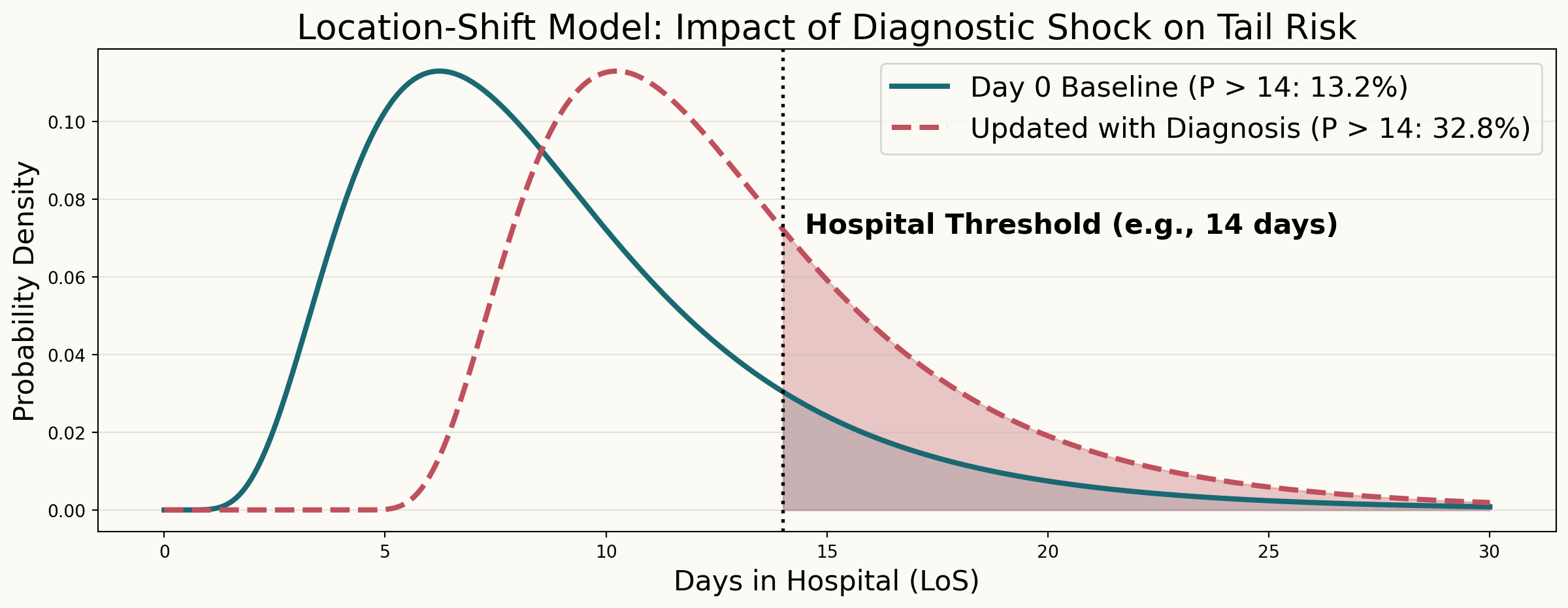
The Causal Location Shift Example

The DML framework treats the diagnostic confirmation as a “shock” that shifts the distribution’s location along the time axis.

🟢 Day 0: Baseline

The “clean-path” prediction based on demographics and only initial information. The shaded area represents the initial risk of becoming a stranded patient.

🔴 Day \(k\): Causal Update

Diagnosis \(\tau_D\) shifts the entire distribution right. The shaded area shows sn increase in the probability of crossing the 14-day threshold.

Counterfactual Simulation & Impact

To prove the framework’s worth, we replay the historical baseline as a simulation:

• Step 1: Run a day-by-day replay of historical patients.
• Step 2: Apply the policy trigger (the “Model Intervention”) the moment a patient hits the risk threshold.
• Step 3: Compute the System Delta (\(\Delta Beds\)):

\[ \Delta \text{Beds} = \sum \text{Actual LoS}_i - \sum \text{Counterfactual LoS}_i \]

This allows us to present decision-makers with a concrete metric: “If we had used this model, we would have reclaimed X bed-days.”

Any questions or thoughts? 💬