# import libraries
import numpy as np
import matplotlib.pyplot as plt
import seaborn as sns
import plotly.express as px
import pandas as pd
# allow max rows to be displayed
pd.set_option('display.max_columns', None)
pd.set_option('display.max_rows', 50)
# ignore warnings
import warnings
warnings.filterwarnings('ignore')
from xgboost import XGBRegressor
from lightgbm import LGBMRegressor
from catboost import CatBoostRegressor
from sklearn.linear_model import LinearRegression, Ridge, Lasso, ElasticNet
from sklearn.model_selection import TimeSeriesSplit, KFold
import pandas as pd
from sklearn.metrics import mean_squared_error, r2_score, mean_absolute_error, root_mean_squared_error
from sklearn.preprocessing import StandardScaler, MinMaxScaler
from sklearn.pipeline import Pipeline
from sklearn.compose import ColumnTransformer
from sklearn.impute import SimpleImputer
from sklearn.ensemble import RandomForestRegressor, HistGradientBoostingRegressor, AdaBoostRegressor, GradientBoostingRegressor
import numpy as np
from cubist import Cubist
from hyperopt import fmin, tpe, hp, Trials, STATUS_OK, space_eval
from hyperopt.pyll import scope
pd.set_option('display.max_rows', 150)
import pickle # for saving and loading models
from statsmodels.tsa.holtwinters import ExponentialSmoothing
from statsmodels.tsa.seasonal import seasonal_decompose, MSTL
from sklearn.tree import DecisionTreeRegressor

from peshbeen.models import (ml_forecaster, ml_bidirect_forecaster, VARModel, MsHmmRegression, MsHmmVar)
from peshbeen.model_selection import (cross_validate,  mv_cross_validate,
                                      cv_tune, mv_cv_tune, prob_param_forecasts,
                                      tune_ets, tune_sarima, ParametricTimeSeriesSplit,
                                      forward_feature_selection, backward_feature_selection,
                                      mv_forward_feature_selection, mv_backward_feature_selection,
                                      hmm_forward_feature_selection, hmm_backward_feature_selection,
                                      hmm_mv_forward_feature_selection, hmm_mv_backward_feature_selection,
                                      hmm_cross_validate, hmm_mv_cross_validate, cv_lag_tune,
                                      cv_hmm_lag_tune)
from peshbeen.statplots import (plot_ccf, plot_PACF_ACF)
from peshbeen.stattools import (unit_root_test, cross_autocorrelation,
                                lr_trend_model, forecast_trend, pacf_strength, ccf_strength)
from peshbeen.transformations import (fourier_terms, rolling_quantile,
                        rolling_mean, rolling_std, expanding_mean, expanding_std,
                        expanding_quantile, expanding_ets, box_cox_transform,
                        back_box_cox_transform,undiff_ts, seasonal_diff, invert_seasonal_diff,
                        nzInterval, zeroCumulative, kfold_target_encoder, target_encoder_for_test)
from peshbeen.metrics import (MAPE, MASE, MSE, MAE, RMSE, SMAPE, CFE, CFE_ABS, WMAPE, SRMSE, RMSSE, SMAE)
from peshbeen.prob_forecast import (ml_prob_forecasts, var_prob_forecasts, hmm_prob_forecasts, ets_prob_forecasts, arima_prob_forecasts, naive_prob_forecasts)
from sktime.transformations.series.boxcox import BoxCoxTransformer
sns.set_context("talk")Probabilistic forecast flow
occup = pd.read_excel('data/occup_train_clean.xlsx', index_col=0)
occup["day_of_week"] = occup.index.day_name()
occup["month"] = occup.index.month_name()
cat_cols = ["day_of_week", "month", "is_holiday"]
cat_col_f = ["day_of_week", "is_holiday"]
hmm_params = {'blake': {'best_states': 2, 'best_lag': 2, 'best_k': 1},
'mulberry': {'best_states': 2, 'best_lag': 3, 'best_k': 1},
'juniper': {'best_states': 2, 'best_lag': 3, 'best_k': 1},
'magnolia': {'best_states': 6, 'best_lag': 3, 'best_k': 2},
'clare': {'best_states': 2, 'best_lag': 3, 'best_k': 1},
'anderson': {'best_states': 2, 'best_lag': 3, 'best_k': 1},
'other': {'best_states': 2, 'best_lag': 2, 'best_k': 2}}
def data_prep_f(ward, fourier_k):
ward_train = occup[[ward, "time"]+cat_col_f]
ft = fourier_terms(start_end_index=(ward_train.index.min(), ward_train.index.max()),
period=365.25, num_terms=fourier_k)
return ward_train.merge(ft, left_index=True, right_index=True, how="left")ward_df= data_prep_f("blake", 1)
train = ward_df.iloc[:-3*84]
test = ward_df.iloc[-3*84:-2*84]
col = "blake"hm_model_ = MsHmmRegression(n_components=2, target_col=col, cat_variables=cat_col_f, lags=2,
random_state=42, n_iter=300, tol=1e-2, ridge=0, verbose=False)
# fit_df = df_[:-360]
hm_model_.fit_em(train)np.float64(360.6669091818735)hm_model_.forecast(H=84, exog=test.drop(columns=[col]))array([18.46521508, 18.19925292, 17.96290128, 17.56453267, 17.06388852,
17.2696804 , 17.59547891, 17.33622422, 17.08008709, 16.89856695,
16.5424621 , 16.08407496, 16.32989381, 16.69418836, 16.47183517,
16.2510934 , 16.10352137, 15.77997885, 15.35282606, 15.62860686,
16.02164419, 15.82686563, 15.63257918, 15.51039003, 15.21120279,
14.80742068, 15.10562875, 15.52018941, 15.34606805, 15.17160892,
15.0684519 , 14.78753487, 14.40129291, 14.7163416 , 15.14707259,
14.98847929, 14.82893279, 14.74009869, 14.47293951, 14.09991391,
14.4276601 , 14.87059137, 14.72372189, 14.57544261, 14.49743816,
14.2406893 , 13.87767216, 14.21504165, 14.66722711, 14.52925804,
14.38954008, 14.31977195, 14.07094787, 13.71555689, 14.06026628,
14.51951721, 14.38835051, 14.25518269, 14.19172285, 13.94897516,
13.59943819, 13.94978834, 14.4144755 , 14.28854888, 14.16043297,
14.10184453, 13.86379508, 13.51879019, 13.87351298, 14.34241979,
14.22056593, 14.09638182, 14.04158985, 13.8072069 , 13.46574373,
13.82388839, 14.29610191, 14.17744415, 14.05634984, 14.00454548,
13.77305194, 13.43438373, 13.79523252, 14.2700628 ])hm_model_.Aarray([[0.6473715 , 0.3526285 ],
[0.44586143, 0.55413857]])hm_model_.posterior.shape, train.shape((2, 1876), (1878, 6))## add 2 NaN in the begining of 2 by 1876 hm_model_.posterior
regime_prob = np.pad(hm_model_.posterior, ((0, 0), (2, 0)), mode='constant', constant_values=np.nan).Tdf_hmm = train[["blake"]]
df_hmm[["regime_1", "regime_2"]] = regime_prob
df_hmm.dropna(inplace=True)df_hmm.to_excel("data/hmm_regime_df.xlsx")hmm_df.info()<class 'pandas.core.frame.DataFrame'>
RangeIndex: 1876 entries, 0 to 1875
Data columns (total 4 columns):
# Column Non-Null Count Dtype
--- ------ -------------- -----
0 Date 1876 non-null datetime64[ns]
1 blake 1876 non-null int64
2 regime_1 1876 non-null float64
3 regime_2 1876 non-null float64
dtypes: datetime64[ns](1), float64(2), int64(1)
memory usage: 58.8 KBimport logging
# Configure basic logging for error tracking
logging.basicConfig(level=logging.INFO, format='%(levelname)s: %(message)s')
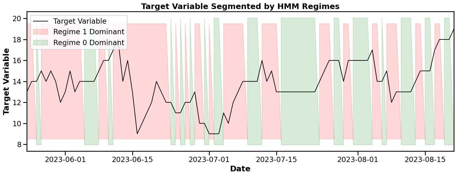
def plot_hmm_regimes(
dates: pd.DatetimeIndex,
target: pd.Series,
posterior_probs: np.ndarray,
threshold: float = 0.5
) -> None:
"""
Plots a time series with background shading indicating the dominant HMM regime.
Dynamically handles cases where the posterior array is shorter than the target series.
Parameters:
dates (pd.DatetimeIndex): The datetime index for the x-axis.
target (pd.Series): The target variable to plot.
posterior_probs (np.ndarray): 2D array of regime probabilities.
threshold (float): Probability threshold to classify a regime. Defaults to 0.5.
"""
try:
fig, ax = plt.subplots(figsize=(15, 6))
# 1. Plot the FULL target variable
ax.plot(dates, target, label='Target Variable', color='black', linewidth=1.5)
is_regime_1 = posterior_probs.values >= threshold
is_regime_0 = ~is_regime_1
# 3. Apply background shading using fill_between
ax.fill_between(
dates,
ax.get_ylim()[0],
ax.get_ylim()[1],
where=is_regime_1,
color='red',
alpha=0.15,
label='Regime 1 Dominant',
interpolate=True
)
ax.fill_between(
dates,
ax.get_ylim()[0],
ax.get_ylim()[1],
where=is_regime_0,
color='green',
alpha=0.15,
label='Regime 0 Dominant',
interpolate=True
)
# 4. Formatting
ax.set_xlabel('Date', fontweight='bold')
ax.set_ylabel('Target Variable', fontweight='bold')
ax.set_title('Target Variable Segmented by HMM Regimes', fontweight='bold')
ax.legend(loc='upper left', frameon=True)
ax.margins(x=0)
plt.tight_layout()
plt.show()
except Exception as e:
logging.error(f"Visualization failed due to: {e}")
raise
plot_hmm_regimes(
dates=df_hmm.index[-90:],
target=df_hmm.loc[:, "blake"][-90:],
posterior_probs=df_hmm["regime_1"][-90:]
)
df_hmm| blake | regime_1 | regime_2 | |
|---|---|---|---|
| Date | |||
| 2018-07-03 | 14 | 2.280415e-15 | 1.000000 |
| 2018-07-04 | 16 | 1.000000e+00 | 0.000000 |
| 2018-07-05 | 15 | 1.000000e+00 | 0.000000 |
| 2018-07-06 | 15 | 4.558888e-03 | 0.995441 |
| 2018-07-07 | 15 | 1.687860e-03 | 0.998312 |
| ... | ... | ... | ... |
| 2023-08-17 | 17 | 1.000000e+00 | 0.000000 |
| 2023-08-18 | 18 | 1.000000e+00 | 0.000000 |
| 2023-08-19 | 18 | 2.963277e-03 | 0.997037 |
| 2023-08-20 | 18 | 4.661595e-03 | 0.995338 |
| 2023-08-21 | 19 | 1.000000e+00 | 0.000000 |
1876 rows × 3 columns
## plot the posterior probabilities on same plot as the target variable so to see regime probabilities but in different axis
fig, ax1 = plt.subplots(figsize=(15, 6))
ax1.plot(train.index[-90:], train["blake"][-90:], label='Target Variable', color='blue')
ax1.set_xlabel('Date')
ax1.set_ylabel('Target Variable', color='blue')
ax1.tick_params(axis='y', labelcolor='blue')
ax2 = ax1.twinx()  # instantiate a second axes that shares the same x-axis
# ax2.plot(train.index[-90:], hm_model_.posterior[0][-90:], label='Regime 1 Probability', color='red')
ax2.plot(train.index[-90:], hm_model_.posterior[1][-90:], label='Regime 2 Probability', color='green')
ax2.set_ylabel('Regime Probabilities', color='black')
ax2.tick_params(axis='y', labelcolor='black')
fig.legend(loc='upper right', bbox_to_anchor=(0.9, 0.9))
plt.title('Target Variable and Regime Probabilities')
plt.show()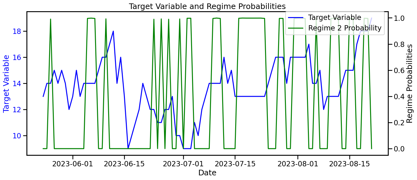
with open('tables/comb_opt_cdf.pkl', 'rb') as f:
    comb_opt_cdf = pickle.load(f)


comb_opt_cdf['total_shortage'] = comb_opt_cdf['total_shortage'].astype(int)

cutoff = 26
markers = ['o', 's', '^', 'D', 'v', 'P', 'X', '*', 'h', '<', '>']

# --------------------------------------------------
# 1. Dominance score: P(0 understaffed days)
# --------------------------------------------------
dominance_score = (
    comb_opt_cdf
    .groupby('Model')['total_shortage']
    .apply(lambda x: (x == 0).mean())
    .sort_values(ascending=False)
)comb_opt_cdf| total_shortage | Model | CDF | |
|---|---|---|---|
| 0 | 0 | AR-MSR | 0.000794 |
| 1 | 0 | AR-MSR | 0.001587 |
| 2 | 0 | AR-MSR | 0.002381 |
| 3 | 0 | AR-MSR | 0.003175 |
| 4 | 0 | AR-MSR | 0.003968 |
| ... | ... | ... | ... |
| 1255 | 27 | AR-MSR (Det-Best Point Forecast) | 0.996825 |
| 1256 | 27 | AR-MSR (Det-Best Point Forecast) | 0.997619 |
| 1257 | 27 | AR-MSR (Det-Best Point Forecast) | 0.998413 |
| 1258 | 28 | AR-MSR (Det-Best Point Forecast) | 0.999206 |
| 1259 | 32 | AR-MSR (Det-Best Point Forecast) | 1.000000 |
12600 rows × 3 columns
g = comb_opt_cdf[comb_opt_cdf['Model'] == "AR-MSR"]comb_opt_cdf| total_shortage | Model | CDF | |
|---|---|---|---|
| 0 | 0 | AR-MSR | 0.000794 |
| 1 | 0 | AR-MSR | 0.001587 |
| 2 | 0 | AR-MSR | 0.002381 |
| 3 | 0 | AR-MSR | 0.003175 |
| 4 | 0 | AR-MSR | 0.003968 |
| ... | ... | ... | ... |
| 1255 | 27 | AR-MSR (Det-Best Point Forecast) | 0.996825 |
| 1256 | 27 | AR-MSR (Det-Best Point Forecast) | 0.997619 |
| 1257 | 27 | AR-MSR (Det-Best Point Forecast) | 0.998413 |
| 1258 | 28 | AR-MSR (Det-Best Point Forecast) | 0.999206 |
| 1259 | 32 | AR-MSR (Det-Best Point Forecast) | 1.000000 |
12600 rows × 3 columns
with open('tables/comb_opt_cdf.pkl', 'rb') as f:
    comb_opt_cdf = pickle.load(f)

plt.figure(figsize=(27, 9))

comb_opt_cdf['total_shortage'] = comb_opt_cdf['total_shortage'].astype(int)

cutoff = 17
markers = ['o', 's', '^', 'D', 'v', 'P', 'X', '*', 'h', '<', '>']

# --------------------------------------------------
# 1. Dominance score: P(0 understaffed days)
# --------------------------------------------------
dominance_score = (
    comb_opt_cdf
    .groupby('Model')['total_shortage']
    .apply(lambda x: (x == 0).mean())
    .sort_values(ascending=False)
)[:-1]

# --------------------------------------------------
# 2. Fixed annotation layout (TOP 5)
# --------------------------------------------------
annot_models = dominance_score.index[:5]
y_positions = np.linspace(0.78, 0.62, len(annot_models))  # evenly spaced

# --------------------------------------------------
# 3. Plot in dominance order
# --------------------------------------------------
for i, model in enumerate(dominance_score.index):

    g = comb_opt_cdf[comb_opt_cdf['Model'] == model]

    x_full = np.arange(
        g['total_shortage'].min(),
        g['total_shortage'].max() + 1
    )

    counts = (
        g['total_shortage']
        .value_counts()
        .reindex(x_full, fill_value=0)
        .sort_index()
    )

    cdf_full = counts.cumsum() / counts.sum()

    mask = x_full <= cutoff
    x_plot = x_full[mask]
    cdf_plot = cdf_full[mask]

    plt.plot(
        x_plot,
        cdf_plot,
        marker=markers[i % len(markers)],
        linestyle='-',
        label=model,
        linewidth=1
    )
    plt.xticks(range(0, cutoff + 1, 1), fontsize=10)


## add vertical line for 0 x axis
plt.axvline(x=0, color='#BF505C', linestyle='--', linewidth=3)

# # --------------------------------------------------
# # 4. Add aligned annotations (axis coordinates)
# # --------------------------------------------------
# ax = plt.gca()

# for y, model in zip(y_positions, annot_models):
#     zero_prob = dominance_score[model]

#     ax.text(
#         0.02, y,                         # left margin in axes coords
#         f"{model}: {zero_prob:.2%}",
#         transform=ax.transAxes,
#         fontsize=24,
#         va='center',
#         ha='left'
#     )

# --------------------------------------------------
# 5. Formatting
# --------------------------------------------------
# plt.annotate(
#     'Zero-Shortage Reliability\nP(0 Understaffed Days):',
#     xy=(0.02, 0.28),
#     xytext=(-0.7, 0.86),
#     fontweight='bold',
#     fontsize=24
# )
plt.xlabel("Number of understaffed days", fontsize=30)
plt.xticks(fontsize=24)
plt.yticks(fontsize=24)
plt.ylabel("Probability of ≤ x Understaffed Days", fontsize=30)
plt.legend(title="Model", fontsize=24)
plt.grid(True)
plt.tight_layout()
plt.show()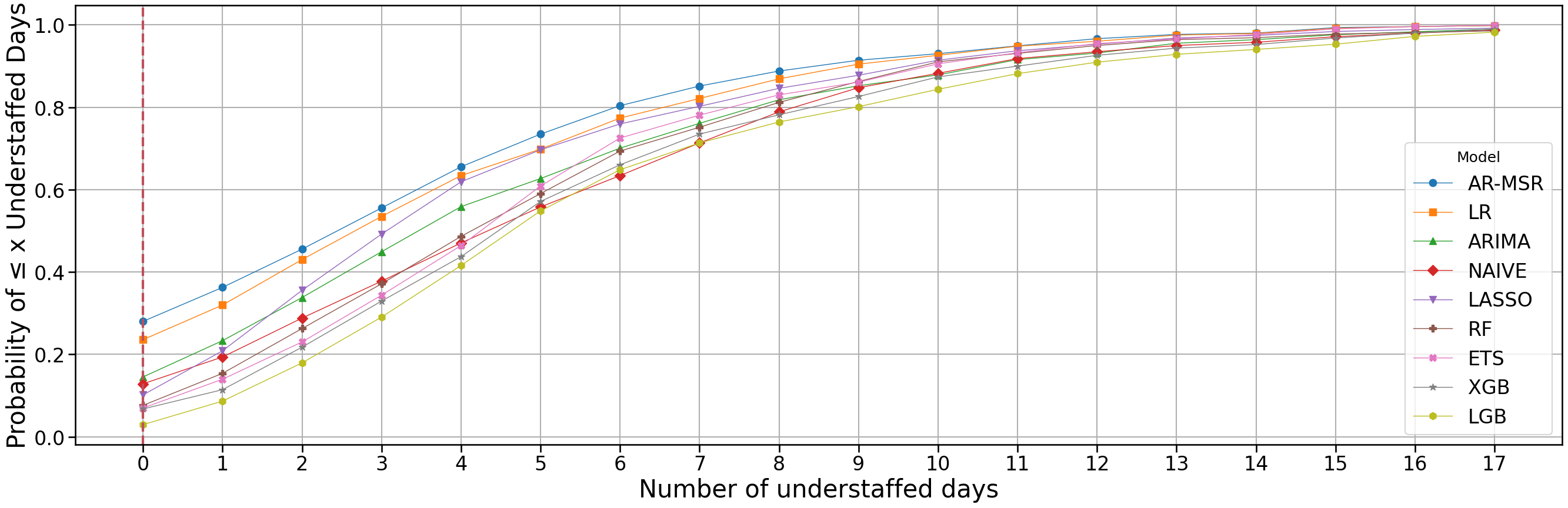
comb_opt_cdf = comb_opt_cdf.iloc[[0, -1]]comb_opt_cdf| total_shortage | Model | CDF | |
|---|---|---|---|
| 0 | 0 | AR-MSR | 0.000794 |
| 1259 | 32 | AR-MSR (Det-Best Point Forecast) | 1.000000 |
# # Save to file
# with open('exp_results/hm_model_.pkl', 'wb') as f:
#     pickle.dump(hm_model_, f)#

# Load from file
with open('exp_results/hm_model_.pkl', 'rb') as f:
    hm_model_ = pickle.load(f)
point_forecasts = hm_model_.forecast(H=84, exog=test.drop(columns=[col]))hmm_prob = hmm_prob_forecasts(model=hm_model_, n_calibration=360, H=84, sliding_window=1, n_iter=100, verbose=False)
hmm_prob.calibrate(train)# # Save to file
# with open('exp_results/hmm_prob.pkl', 'wb') as f:
# pickle.dump(hmm_prob, f)#
# Load from file
with open('exp_results/hmm_prob.pkl', 'rb') as f:
hmm_prob = pickle.load(f)boost = hmm_prob.simulate_correlated_forecasts(train, samples=1000, future_exog=test.drop(columns=[col]))prob_forecasts = boost.correlated_forecasts## Generate point forecasts
## Generate probabilistic forecasts
from datetime import timedelta
scenarios_hmm = np.array(prob_forecasts)
## plot scenarios agains train and test
plt.figure(figsize=(12, 6))
plt.plot(train[col].index[-120:], train[col][-120:], label='Train', color='C0')
plt.plot(test.index, test[col], label='Actual', color='C2', linewidth=2, alpha=1)
plt.plot(test.index, point_forecasts, label='Point Forecast', color='C3')
# Define decision time (start of forecast horizon)
decision_time = test.index[0]+ timedelta(days=-1) # first day of test/forecast period
# for i in range(scenarios_hmm.shape[0]-1):
# plt.plot(test.index, scenarios_hmm[i], color='C7', alpha=0.1)
# plt.plot(test.index, scenarios_hmm[-1], color='C7', alpha=0.1, label ='All Scenarios (1000)')
# 1. Vertical dashed line
plt.axvline(decision_time, color='black', linestyle='--', linewidth=1.5)
# 2. "Decision time" label at top
plt.text(
decision_time,
plt.ylim()[1] * 0.98,
"Decision time",
ha='center',
va='top',
fontsize=12,
fontweight='bold',
color='black'
)
# 3. Explanation text box
plt.text(
decision_time,
plt.ylim()[1] * 0.90,
"Decision:\nHow many nurses\nshould I schedule\nfor each day of next 42-84 days of forecasting horizon?",
ha='center',
va='top',
fontsize=11,
color='black',
bbox=dict(facecolor='white', alpha=0.4, edgecolor='none')
)
# Choose a low y-level automatically (5% above bottom of plot)
hline_y = plt.ylim()[0] + 0.05 * (plt.ylim()[1] - plt.ylim()[0])
# Horizontal line spanning forecasting period
plt.hlines(
y=hline_y,
xmin=test.index[42],
xmax=test.index[-1],
color='C5',
linestyle='--',
linewidth=2,
alpha=0.8
)
# Label next to the horizontal line
plt.text(
test.index[62],
hline_y,
"Uncertainty in occupancy levels\nfor the next 42 days",
ha='center',
va='bottom',
fontsize=11,
color='black'
)
plt.ylabel('Occupancy')
plt.xlabel('Date')
plt.grid(True)
plt.legend(fontsize=12)
plt.show()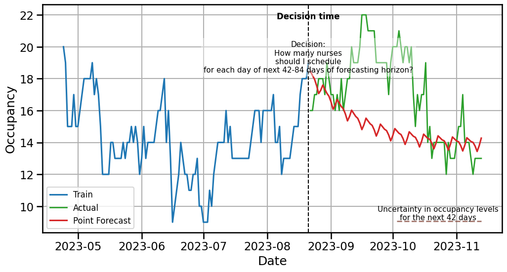
## Generate point forecasts
## Generate probabilistic forecasts
from datetime import timedelta


scenarios_hmm = np.array(prob_forecasts)

## plot scenarios agains train and test
plt.figure(figsize=(12, 6))
plt.plot(train[col].index[-120:], train[col][-120:], label='Train', color='C0')
plt.plot(test.index, test[col], label='Actual', color='C2', linewidth=2, alpha=1)
plt.plot(test.index, point_forecasts, label='Point Forecast', color='C3')
# Define decision time (start of forecast horizon)
decision_time = test.index[0]+ timedelta(days=-1)  # first day of test/forecast period
# for i in range(scenarios_hmm[0:3].shape[0]-1):
#     plt.plot(test.index, scenarios_hmm[i], color='C7', alpha=0.5)
plt.plot(test.index, scenarios_hmm[-1], color='C7', alpha=0.5, label ='All Scenarios (1000)')

# 1. Vertical dashed line
plt.axvline(decision_time, color='black', linestyle='--', linewidth=1.5)

# 2. "Decision time" label at top
plt.text(
    decision_time,
    plt.ylim()[1] * 0.98,
    "Decision time",
    ha='center',
    va='top',
    fontsize=12,
    fontweight='bold',
    color='black'
)

# 3. Explanation text box
plt.text(
    decision_time,
    plt.ylim()[1] * 0.90,
    "Decision:\nHow many nurses\nshould I schedule\nfor each day of next 42-84 days of forecasting horizon?",
    ha='center',
    va='top',
    fontsize=11,
    color='black',
    bbox=dict(facecolor='white', alpha=0.4, edgecolor='none')
)


# Choose a low y-level automatically (5% above bottom of plot)
hline_y = plt.ylim()[0] + 0.05 * (plt.ylim()[1] - plt.ylim()[0])

# Horizontal line spanning forecasting period
plt.hlines(
    y=hline_y,
    xmin=test.index[42],
    xmax=test.index[-1],
    color='C5',
    linestyle='--',
    linewidth=2,
    alpha=0.8
)

# Label next to the horizontal line
plt.text(
    test.index[62],
    hline_y,
    "Uncertainty in occupancy levels\nfor the next 42 days",
    ha='center',
    va='bottom',
    fontsize=11,
    color='black'
)


plt.ylabel('Occupancy')
plt.xlabel('Date')
plt.grid(True)
plt.legend(fontsize=12)
plt.show()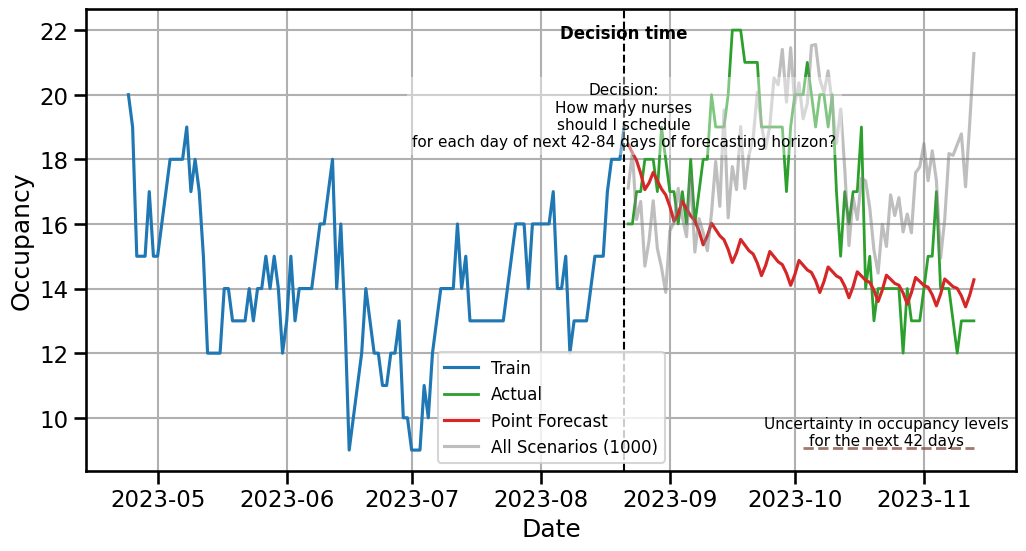
tables
from great_tables import *f_metrics = pd.read_csv("tables/model_ward_sgain_forecasts.csv")f_metrics.replace({"model": {"PermEntropy": ""}}, inplace=True)f_metrics| model | Ward A | Ward B | Ward C | Ward D | Ward E | Ward F | Ward G | overall | metric | |
|---|---|---|---|---|---|---|---|---|---|---|
| 0 | AR-MSR | 3.373633 | 4.947921 | 3.260366 | 3.910015 | 2.800352 | 3.782174 | 2.105290 | 3.454250 | RMSE |
| 1 | LASSO | 3.793185 | 5.341442 | 4.075063 | 2.318951 | 3.067318 | 3.685791 | 2.084345 | 3.480871 | RMSE |
| 2 | LR | 3.623391 | 5.664509 | 3.700904 | 2.199278 | 3.335767 | 3.983707 | 2.080061 | 3.512517 | RMSE |
| 3 | RF | 3.956461 | 5.071211 | 4.382106 | 2.639701 | 2.867912 | 4.090270 | 2.098558 | 3.586603 | RMSE |
| 4 | ETS | 3.698820 | 5.486072 | 3.888890 | 2.606520 | 3.602168 | 3.948612 | 2.048124 | 3.611315 | RMSE |
| 5 | TimeGPT | 4.095112 | 5.507926 | 3.779924 | 2.758942 | 3.407333 | 3.660007 | 2.513029 | 3.674610 | RMSE |
| 6 | ARIMA | 3.662656 | 5.729906 | 4.063827 | 2.463221 | 3.730140 | 3.975073 | 2.198374 | 3.689028 | RMSE |
| 7 | NAIVE | 4.260987 | 5.399300 | 3.892615 | 2.899999 | 3.448369 | 3.706992 | 2.580958 | 3.741317 | RMSE |
| 8 | XGB | 4.224786 | 5.253307 | 5.149105 | 2.571125 | 3.643394 | 3.943408 | 2.011702 | 3.828118 | RMSE |
| 9 | LGB | 3.984276 | 5.500140 | 4.400395 | 4.086323 | 3.289454 | 3.862070 | 1.999413 | 3.874582 | RMSE |
| 10 | AR-MSR | 1.045588 | 1.525511 | 0.964952 | 0.868996 | 0.871215 | 1.215376 | 0.600589 | 1.013175 | Pinball |
| 11 | LR | 1.012719 | 1.498275 | 0.963025 | 0.968045 | 0.845042 | 1.294412 | 0.611702 | 1.027603 | Pinball |
| 12 | LASSO | 1.136555 | 1.606141 | 1.058391 | 0.912206 | 0.874879 | 1.190900 | 0.610077 | 1.055593 | Pinball |
| 13 | RF | 1.249672 | 1.640816 | 1.221365 | 0.916781 | 0.865144 | 1.353165 | 0.637384 | 1.126332 | Pinball |
| 14 | XGB | 1.226932 | 1.677229 | 1.325663 | 0.813778 | 0.992039 | 1.348910 | 0.633346 | 1.145414 | Pinball |
| 15 | ETS | 1.245543 | 1.806563 | 1.107668 | 0.942603 | 1.091017 | 1.351288 | 0.644271 | 1.169851 | Pinball |
| 16 | NAIVE | 1.383129 | 1.746438 | 1.221968 | 0.965408 | 1.100163 | 1.128023 | 0.803762 | 1.192699 | Pinball |
| 17 | ARIMA | 1.163442 | 1.866146 | 1.277825 | 1.000289 | 1.187604 | 1.209706 | 0.668664 | 1.196239 | Pinball |
| 18 | LGB | 1.186391 | 1.833974 | 1.185235 | 1.414645 | 0.995072 | 1.304311 | 0.631901 | 1.221647 | Pinball |
| 19 | TimeGPT | 1.448103 | 1.955222 | 1.334803 | 0.976975 | 1.238214 | 1.294727 | 0.867477 | 1.302217 | Pinball |
| 20 | 0.760015 | 0.723240 | 0.712319 | 0.657460 | 0.613129 | 0.613726 | 0.563251 | 0.663306 | PermEntropy | |
| 21 | AR-MSR | 0.115079 | 1.617460 | 0.422222 | 0.010317 | 0.404762 | 0.979365 | 0.162698 | 3.711905 | STO |
| 22 | LR | 0.214286 | 1.712698 | 0.512698 | 0.003968 | 0.238889 | 1.169841 | 0.155556 | 4.007937 | STO |
| 23 | LASSO | 0.429365 | 1.565873 | 0.938889 | 0.009524 | 0.160317 | 1.280159 | 0.158730 | 4.542857 | STO |
| 24 | ARIMA | 0.731746 | 1.737302 | 0.352381 | 0.015873 | 0.535714 | 1.250000 | 0.312698 | 4.935714 | STO |
| 25 | ETS | 0.270635 | 1.139683 | 0.681746 | 0.008730 | 1.371429 | 1.595238 | 0.158730 | 5.226190 | STO |
| 26 | RF | 0.442063 | 1.718254 | 1.230159 | 0.068254 | 0.469048 | 1.220635 | 0.144444 | 5.292857 | STO |
| 27 | NAIVE | 1.136508 | 1.582540 | 0.409524 | 0.108730 | 0.534921 | 1.212698 | 0.449206 | 5.434127 | STO |
| 28 | XGB | 0.595238 | 1.227778 | 1.391270 | 0.024603 | 0.743651 | 1.595238 | 0.153968 | 5.731746 | STO |
| 29 | LGB | 0.557143 | 1.619048 | 1.284921 | 0.013492 | 0.903968 | 1.595238 | 0.164286 | 6.138095 | STO |
| 30 | AR-MSR-PointForecasts | 1.165873 | 3.584127 | 1.342063 | 0.138889 | 1.079365 | 1.595238 | 0.153968 | 9.059524 | STO |
| 31 | AR-MSR | 833.571429 | 1333.650794 | 836.190476 | 657.698413 | 669.841270 | 822.857143 | 447.857143 | 5601.666667 | VSS |
| 32 | LASSO | 883.253968 | 1319.126984 | 931.825397 | 676.349206 | 615.555556 | 841.349206 | 446.825397 | 5714.285714 | VSS |
| 33 | LR | 849.047619 | 1340.476190 | 850.634921 | 739.603175 | 641.666667 | 870.476190 | 452.063492 | 5743.968253 | VSS |
| 34 | ETS | 858.968254 | 1261.428571 | 883.571429 | 650.079365 | 811.428571 | 878.571429 | 447.301587 | 5791.349206 | VSS |
| 35 | RF | 883.095238 | 1329.761905 | 987.777778 | 653.968254 | 675.793651 | 836.984127 | 453.333333 | 5820.714286 | VSS |
| 36 | XGB | 910.476190 | 1262.936508 | 1017.380952 | 633.253968 | 745.476190 | 878.571429 | 446.190476 | 5894.285714 | VSS |
| 37 | ARIMA | 932.698413 | 1398.968254 | 909.206349 | 699.841270 | 725.793651 | 845.158730 | 494.285715 | 6005.952382 | VSS |
| 38 | NAIVE | 1041.746032 | 1376.666667 | 903.174603 | 661.190476 | 730.317460 | 817.619048 | 555.396825 | 6086.111111 | VSS |
| 39 | LGB | 899.047619 | 1353.968254 | 1005.476190 | 766.428571 | 750.079365 | 878.571429 | 448.492063 | 6102.063492 | VSS |
| 40 | AR-MSR-PointForecasts | 1022.619048 | 1746.984127 | 1006.746032 | 613.095238 | 768.571429 | 878.571429 | 446.190476 | 6482.777778 | VSS |
f_metrics = pd.read_csv("tables/model_ward_sgain_forecasts.csv")
group_map = {
    "RMSE": "Point Forecast (RMSE)",
    "Pinball": "Probabilistic (Pinball Loss)",
    "PermEntropy": "Permutation Entropy",
    "STO": "Average Understaffed Number of Patients",
    "VSS": "Value of Stochastic Solution"
}

f_metrics_view = f_metrics.assign(metric=f_metrics["metric"].replace(group_map))

GT(f_metrics_view).tab_stub(groupname_col="metric").tab_style(
    style=style.fill(color="#FBFAF4"),
    locations=loc.body()
).tab_style(
    style=style.fill(color="#20808D"),
    locations=loc.column_header()
).tab_style(
    style=style.text(color="#FBFAF4", weight="bold"),
    locations=loc.column_labels()
).tab_style(
    # Targeting the row group labels specifically
    style=[
        style.fill(color="#20808D"),
        style.text(color="#FBFAF4", weight="bold")
    ],
    locations=loc.row_groups()
).tab_style(
        style=style.text(size="38px", weight="bold"),
        locations=loc.column_labels()
    ).tab_style(
        style=style.text(size="36px"),
        locations=loc.body()
)| model | Ward A | Ward B | Ward C | Ward D | Ward E | Ward F | Ward G | overall |
|---|---|---|---|---|---|---|---|---|
| Point Forecast (RMSE) | ||||||||
| AR-MSR | 3.3736325222806594 | 4.9479213593117475 | 3.2603664196995603 | 3.910014573851342 | 2.8003516710737717 | 3.78217417220872 | 2.1052900735969664 | 3.4542501131461094 |
| LASSO | 3.793185217596648 | 5.3414415585736315 | 4.075062540070708 | 2.318951228444537 | 3.0673181364467195 | 3.6857912371812858 | 2.0843451115078797 | 3.480870718545915 |
| LR | 3.6233911417590305 | 5.664509055807773 | 3.7009041794708417 | 2.199278262453863 | 3.335766512790936 | 3.983706623960853 | 2.0800614715029813 | 3.51251674967804 |
| RF | 3.956460859156175 | 5.071210553765478 | 4.382106481001265 | 2.639701270318182 | 2.867911956206467 | 4.090270065963361 | 2.09855798820284 | 3.586602739230538 |
| ETS | 3.698820423579899 | 5.486072037184399 | 3.8888902836483767 | 2.6065201189737772 | 3.602168307178825 | 3.948612055940692 | 2.0481244272801713 | 3.611315379112306 |
| TimeGPT | 4.095111878591425 | 5.507925562611942 | 3.779924129775609 | 2.758941878046337 | 3.407332852275019 | 3.660006772990124 | 2.5130292584559366 | 3.674610333249484 |
| ARIMA | 3.662655832476581 | 5.729905546461908 | 4.063826627378163 | 2.463220867810203 | 3.730139616106371 | 3.975072518826525 | 2.1983735929913717 | 3.689027800293018 |
| NAIVE | 4.260987040964574 | 5.399299752142806 | 3.8926151003546345 | 2.8999988369509304 | 3.4483687089421675 | 3.7069920924559177 | 2.5809578448760058 | 3.7413170538124336 |
| XGB | 4.22478572823843 | 5.253307070988415 | 5.14910494514314 | 2.5711249060260664 | 3.643394453862358 | 3.943407713572969 | 2.011702066389987 | 3.828118126317338 |
| LGB | 3.9842762875188433 | 5.500139533944931 | 4.4003954354861134 | 4.0863227950048095 | 3.28945411312878 | 3.862069763025887 | 1.9994134519250544 | 3.8745816257192023 |
| Probabilistic (Pinball Loss) | ||||||||
| AR-MSR | 1.0455875579861142 | 1.5255110475719946 | 0.9649518069053143 | 0.8689964743838985 | 0.8712152071667197 | 1.2153756722484013 | 0.6005890560222211 | 1.0131752603263806 |
| LR | 1.0127193110566717 | 1.4982747879743534 | 0.9630251847086618 | 0.968044519050438 | 0.8450424718575041 | 1.2944118782428118 | 0.611701816919458 | 1.0276028528299856 |
| LASSO | 1.1365554539073948 | 1.60614119344363 | 1.058390926918535 | 0.9122055708463676 | 0.8748794130505652 | 1.190900129362254 | 0.6100767774966529 | 1.0555927807179144 |
| RF | 1.2496724479447865 | 1.640816120670067 | 1.221364718972858 | 0.9167805244756492 | 0.8651444806631923 | 1.3531649571401048 | 0.63738417749596 | 1.1263324896232312 |
| XGB | 1.226931581221036 | 1.6772289492956132 | 1.3256634397400446 | 0.813778291420804 | 0.9920388979708644 | 1.3489098199301053 | 0.6333462498260695 | 1.145413889914934 |
| ETS | 1.245543412227771 | 1.8065633587027037 | 1.107667894194592 | 0.9426031403408556 | 1.091016965316723 | 1.3512878351742563 | 0.6442709168543923 | 1.1698505032587565 |
| NAIVE | 1.3831290847885516 | 1.7464382527182014 | 1.2219682238106846 | 0.965408082750928 | 1.1001625417693714 | 1.1280228171112354 | 0.803762038793292 | 1.1926987202488948 |
| ARIMA | 1.1634417415669212 | 1.866146428689427 | 1.27782549302118 | 1.0002886569303275 | 1.187604198455248 | 1.2097061055732412 | 0.668663566465396 | 1.1962394558145346 |
| LGB | 1.1863909289942072 | 1.8339742459478732 | 1.1852349778567757 | 1.4146446159996908 | 0.9950716168133968 | 1.304311002239472 | 0.6319007856533069 | 1.221646881929246 |
| TimeGPT | 1.448102945413886 | 1.9552222822739664 | 1.3348032419839704 | 0.976974874457276 | 1.2382143427588694 | 1.294727288827358 | 0.8674771408778873 | 1.302217445227602 |
| Permutation Entropy | ||||||||
| PermEntropy | 0.7600151178826429 | 0.723239948259235 | 0.7123187468675354 | 0.657460223717832 | 0.6131288328640623 | 0.6137260493073763 | 0.5632510909790247 | 0.6633057156968155 |
| Average Understaffed Number of Patients | ||||||||
| AR-MSR | 0.115079365079365 | 1.6174603174603177 | 0.4222222222222222 | 0.0103174603174603 | 0.4047619047619047 | 0.9793650793650792 | 0.1626984126984127 | 3.711904761904762 |
| LR | 0.2142857142857142 | 1.7126984107051404 | 0.5126984126984127 | 0.0039682539682539 | 0.2388888888888889 | 1.16984126984127 | 0.1555555555555555 | 4.007936505943236 |
| LASSO | 0.4293650793650793 | 1.565873015873016 | 0.9388888888888888 | 0.0095238095238095 | 0.1603174603174603 | 1.28015873015873 | 0.1587301587301587 | 4.542857142857143 |
| ARIMA | 0.7317460317460317 | 1.7373015873015871 | 0.3523809523809524 | 0.0158730158730158 | 0.5357142857142857 | 1.25 | 0.3126984167550957 | 4.935714289770968 |
| ETS | 0.2706349206349206 | 1.1396825396825396 | 0.6817460317460318 | 0.0087301587301587 | 1.3714285714285714 | 1.5952380952380951 | 0.1587301587301587 | 5.226190476190476 |
| RF | 0.442063492063492 | 1.718253968253968 | 1.2301587301587302 | 0.0682539682539682 | 0.469047619047619 | 1.2206349206349207 | 0.1444444444444444 | 5.292857142857143 |
| NAIVE | 1.1365079365079365 | 1.5825396825396825 | 0.4095238095238095 | 0.1087301587301587 | 0.5349206349206349 | 1.2126984126984126 | 0.4492063492063492 | 5.434126984126984 |
| XGB | 0.5952380952380952 | 1.227777777777778 | 1.3912698412698412 | 0.0246031746031746 | 0.7436507936507937 | 1.5952380952380951 | 0.1539682539682539 | 5.731746031746032 |
| LGB | 0.5571428571428572 | 1.619047619047619 | 1.284920634920635 | 0.0134920634920634 | 0.903968253968254 | 1.5952380952380951 | 0.1642857142857142 | 6.1380952380952385 |
| AR-MSR-PointForecasts | 1.165873015873016 | 3.5841269841269843 | 1.342063492063492 | 0.1388888888888889 | 1.0793650793650793 | 1.5952380952380951 | 0.1539682539682539 | 9.05952380952381 |
| Value of Stochastic Solution | ||||||||
| AR-MSR | 833.5714285714286 | 1333.6507936507935 | 836.1904761904761 | 657.6984126984127 | 669.8412698412699 | 822.8571428571429 | 447.8571428571428 | 5601.666666666667 |
| LASSO | 883.2539682539683 | 1319.126984126984 | 931.8253968253968 | 676.3492063492064 | 615.5555555555555 | 841.3492063492064 | 446.8253968253968 | 5714.285714285715 |
| LR | 849.047619047619 | 1340.4761899579398 | 850.6349206349206 | 739.6031746031746 | 641.6666666666666 | 870.4761904761905 | 452.0634920634921 | 5743.968253450003 |
| ETS | 858.968253968254 | 1261.428571428571 | 883.5714285714286 | 650.0793650793651 | 811.4285714285714 | 878.5714285714286 | 447.3015873015873 | 5791.349206349207 |
| RF | 883.0952380952381 | 1329.7619047619048 | 987.7777777777778 | 653.968253968254 | 675.7936507936508 | 836.984126984127 | 453.3333333333333 | 5820.714285714285 |
| XGB | 910.4761904761904 | 1262.936507936508 | 1017.3809523809524 | 633.2539682539683 | 745.4761904761905 | 878.5714285714286 | 446.1904761904762 | 5894.285714285715 |
| ARIMA | 932.6984126984128 | 1398.968253968254 | 909.2063492063492 | 699.8412698412699 | 725.7936507936508 | 845.1587301587301 | 494.285715299885 | 6005.952381966551 |
| NAIVE | 1041.7460317460318 | 1376.6666666666667 | 903.1746031746032 | 661.1904761904761 | 730.3174603174604 | 817.6190476190476 | 555.3968253968254 | 6086.111111111111 |
| LGB | 899.047619047619 | 1353.968253968254 | 1005.4761904761904 | 766.4285714285714 | 750.0793650793651 | 878.5714285714286 | 448.4920634920635 | 6102.063492063492 |
| AR-MSR-PointForecasts | 1022.6190476190476 | 1746.984126984127 | 1006.7460317460316 | 613.0952380952381 | 768.5714285714286 | 878.5714285714286 | 446.1904761904762 | 6482.777777777777 |