


Winner • Joint 1st
SPHERE-PPL Forecasting Contest • NHS Acute Patient Harm (1–5 Day Category)
Markov-Switching AutoRegressive Regression (MS-ARR) Forecasting Severe Acute Patient Harm Resulting from Emergency Department Delays
Winning Team • Data Lab for Social Good
Prof. Bahman Rostami-Tabar
Professor of Analytics & Decision Sciences
Director, Data Lab for Social Good Research Group
Cardiff Business School, Cardiff University
Cardiff Business School, Cardiff University
Mustafa Aslan
PhD Student
Data Lab for Social Good Research Group
Cardiff Business School, Cardiff University
Cardiff Business School, Cardiff University
Harsha Halgamuwe Hewage
PhD Student
Data Lab for Social Good Research Group
Cardiff Business School, Cardiff University
Cardiff Business School, Cardiff University
23 September 2026
Outline
- What Are We Forecasting?
- Model: Markov-Switching AutoRegressive Regression (MS-ARR)
- Model Results
- Data Preparation & How to Forecast Next Days in Python
- Beyond Point Forecasting
Outline
- What Are We Forecasting?
- Model: Markov-Switching AutoRegressive Regression (MS-ARR)
- Model Results
- Data Preparation & How to Forecast Next Days in Python
- Beyond Point Forecasting
What Are We Forecasting?
The Target Outcome Variable
- Target Variable (\(y_t\)): Daily Estimated Avoidable Deaths (EAD) \[\text{EAD}_t = \sum_{i \in \text{Admissions}_t} \Big[ p_i(\text{delay}_i, \mathbf{z}_i) - p_i(0, \mathbf{z}_i) \Big]\]
- \(\mathbf{z}_i\): Baseline patient case-mix vector (age, triage acuity, comorbidities).
- \(\text{delay}_i\): Hours delayed in ED awaiting an inpatient bed.
- \(p_i(\cdot)\): 30-day mortality risk
- Forecasting Objective: Daily forecasts over a 10-day horizon (\(h = 1, \dots, 10\) days ahead) using near-real-time operational data.
- Evaluation: Days 1–5 (\(\text{MSE}_{1\text{–}5\text{d}}\)) & Days 6–10 (\(\text{MSE}_{6\text{–}10\text{d}}\)).
Key Forecasting Constraints & Rules
- Midday Forecasting Cut-off: Forecasts for days \(D+1\) to \(D+10\) can only use information available up to midday on day \(D\).
- Strict 3-Day Reporting Lag:
Because of verification lags, the target variable \(y\) is only known up to \(D-3\).- On Day \(D\), the most recent observed target value is \(y_{D-3}\).
- Sliding Evaluation Windows: 131 sliding 10-day forecast windows evaluated over the hold-out test period (October 2025 – March 2026).
Outline
- What Are We Forecasting?
- Model: Markov-Switching AutoRegressive Regression (MS-ARR)
- Model Results
- Data Preparation & How to Forecast Next Days in Python
- Beyond Point Forecasting
MS-ARR Formulation
\[ y_t \mid (r_t = r) = \beta_{0}^{(r)} + \sum_{i=1}^{p} \beta_{i}^{(r)} \, y_{t-i} + \sum_{m=p+1}^{M} \beta_{m}^{(r)} X_{tm} + \epsilon_t \]
where \(\epsilon_t \sim \mathcal{N}\!\left(0, \sigma_r^2\right)\) is \(i.i.d.\) noise.
- To model regime dynamics, we assume that the latent process \(\{r_t\}\) satisfies the Markov property:
\[ P(r_t = j \mid r_{1:t-1}) = P(r_t = j \mid r_{t-1}), \qquad j \in \mathcal{R}, \; t \ge 2. \]
- The transition probabilities are defined as:
\[ P = \begin{pmatrix} p_{11} & \cdots & p_{1K} \\ \vdots & \ddots & \vdots \\ p_{K1} & \cdots & p_{KK} \end{pmatrix}. \]
Notation & Definitions
- \(y_t\) is the observed number of avoidable deaths at time \(t\),
- \(r_t\) is the unobserved (hidden) regime at time \(t\),
- \(X_{tm}\) are the exogenous predictors.
- \(\beta_{0}^{(r)}\) is the regime-specific intercept
- \(\beta_{i}^{(r)}\) are the autoregressive coefficients associated with the \(i\)-th lag in regime \(r\)
- \(\beta_{m}^{(r)}\) are the coefficients for the exogenous covariates in regime \(r\)
- \(K\) is the total number of regimes. Set of regimes is \(\mathcal{R} = \{1, 2, \ldots, K\}\).
Parameter Estimation of MS-ARR
Model parameters are estimated using the Expectation–Maximization (EM) algorithm, which iteratively refines the parameter vector
\[ \theta = \{\beta^{(r)}, \sigma_r^2, P, \pi \}_{r \in \mathcal{R}} \]
by maximising the likelihood of the observed EAD time series \(y_{1:T} = (y_1, \ldots, y_T)\).
EM Algorithm (The Forward-Backward Algorithm - Baum-Welch)
Let \(k\) denote the iteration index. The EM algorithm proceeds as follows:
\[ \begin{aligned} &\textbf{E-step:} \\[4pt] &\quad Q(\theta \mid \theta^{(k)}) = \mathbb{E}_{\,r_{1:T} \mid y_{1:T},\, \theta^{(k)}} \left[ \log p(y_{1:T}, r_{1:T} \mid \theta) \right] \\[14pt] &\textbf{M-step:} \\[4pt] &\quad \theta^{(k+1)} = \arg\max_{\theta}\, Q(\theta \mid \theta^{(k)}) \\[14pt] &\textbf{Iterate until convergence:} \\[4pt] &\quad \theta^{(0)} \;\rightarrow\; \text{E-step} \;\rightarrow\; \text{M-step} \;\rightarrow\; \theta^{(1)} \;\rightarrow\; \cdots \;\rightarrow\; \theta^{(k+1)} \end{aligned} \]
Forecasting with MS-ARR
\(P(r_T = i \mid O_{1:T})\) denote the filtered probability of being in regime \(i\) at time \(T\). The \(h\)-step-ahead regime probabilities are obtained according to
\[ P(r_{T+h} = j \mid O_{1:T}) = \sum_{i=1}^{K} P(r_{T+h-1} = i \mid O_{1:T}) \, p_{ij}, \qquad h \ge 1. \]
Conditional on regime \(r_{T+h} = r\), the \(h\)-step-ahead forecast of the occupancy process is obtained from the regime-specific autoregressive model,
\[ \hat{y}_{T+h}^{(r)} = \beta_{0}^{(r)} + \sum_{i=1}^{p} \beta_{i}^{(r)} \, y_{T+h-i} + \sum_{m=1}^{M} \beta_{p+m}^{(r)} \, X_{T+h,m}, \]
The final point forecast at horizon \(h\) is computed as a probability-weighted average of the regime-specific forecasts,
\[ \hat{y}_{T+h} = \sum_{r=1}^{K} P(r_{T+h} = r \mid y_{1:T}) \, \hat{y}_{T+h}^{(r)}. \]
Outline
- What We Are Forecasting
- Model: Markov-Switching AutoRegressive Regression (MS-ARR)
- Model Results
- Data Preparation & How to Forecast Next Days in Python
- Beyond Point Forecasting
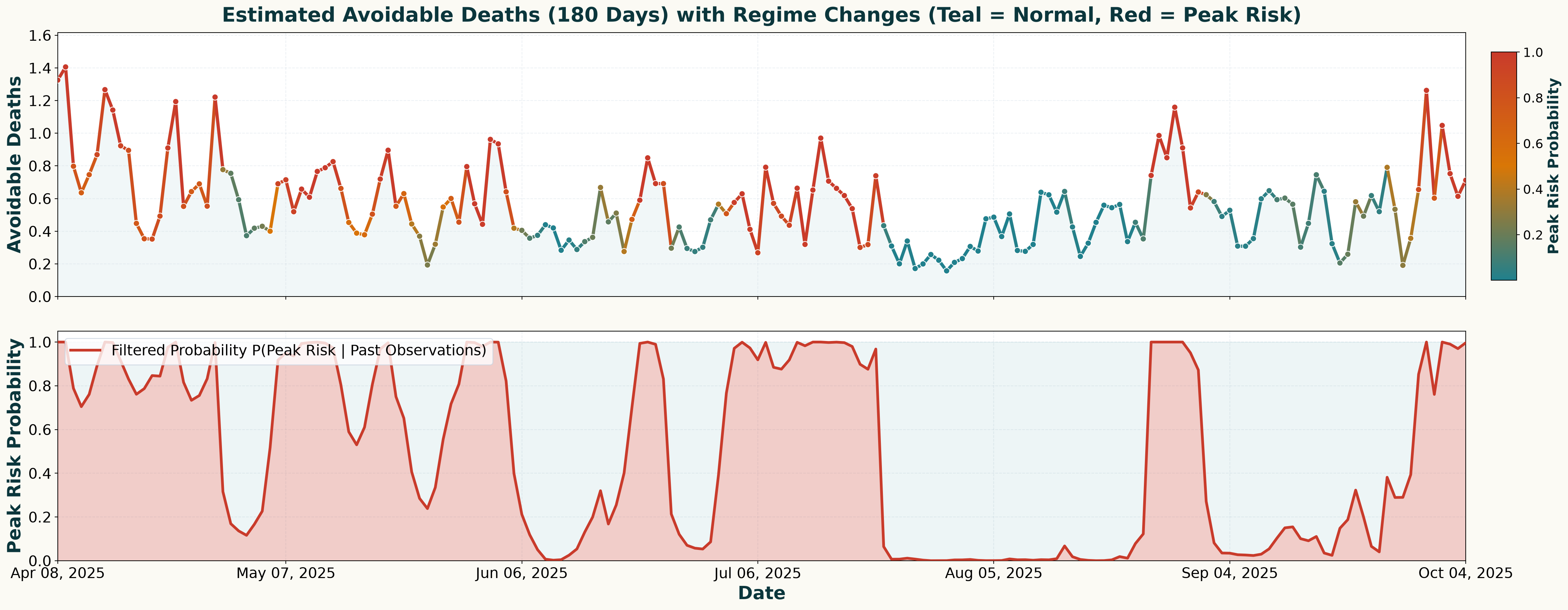
Regime Switches in EAD History
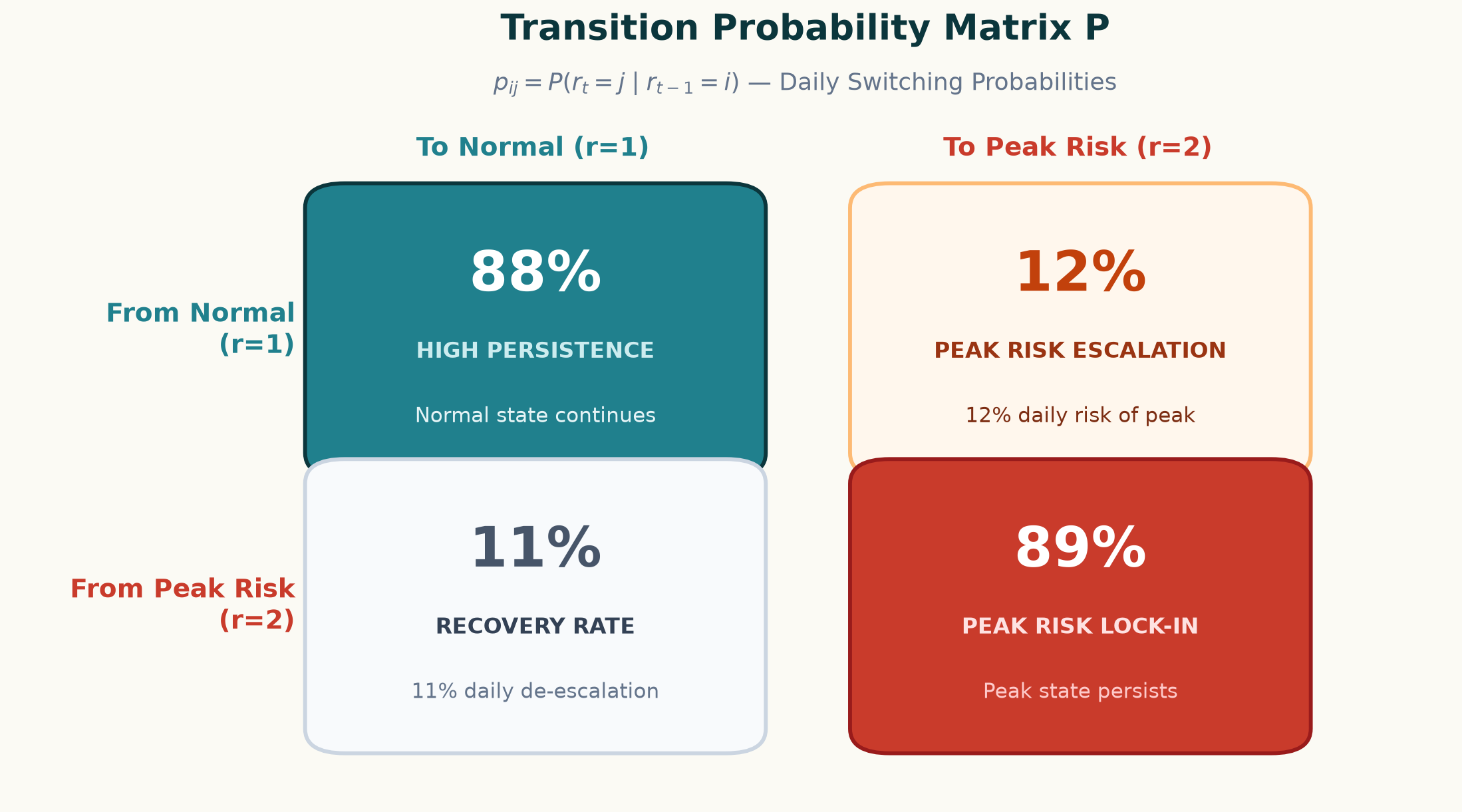
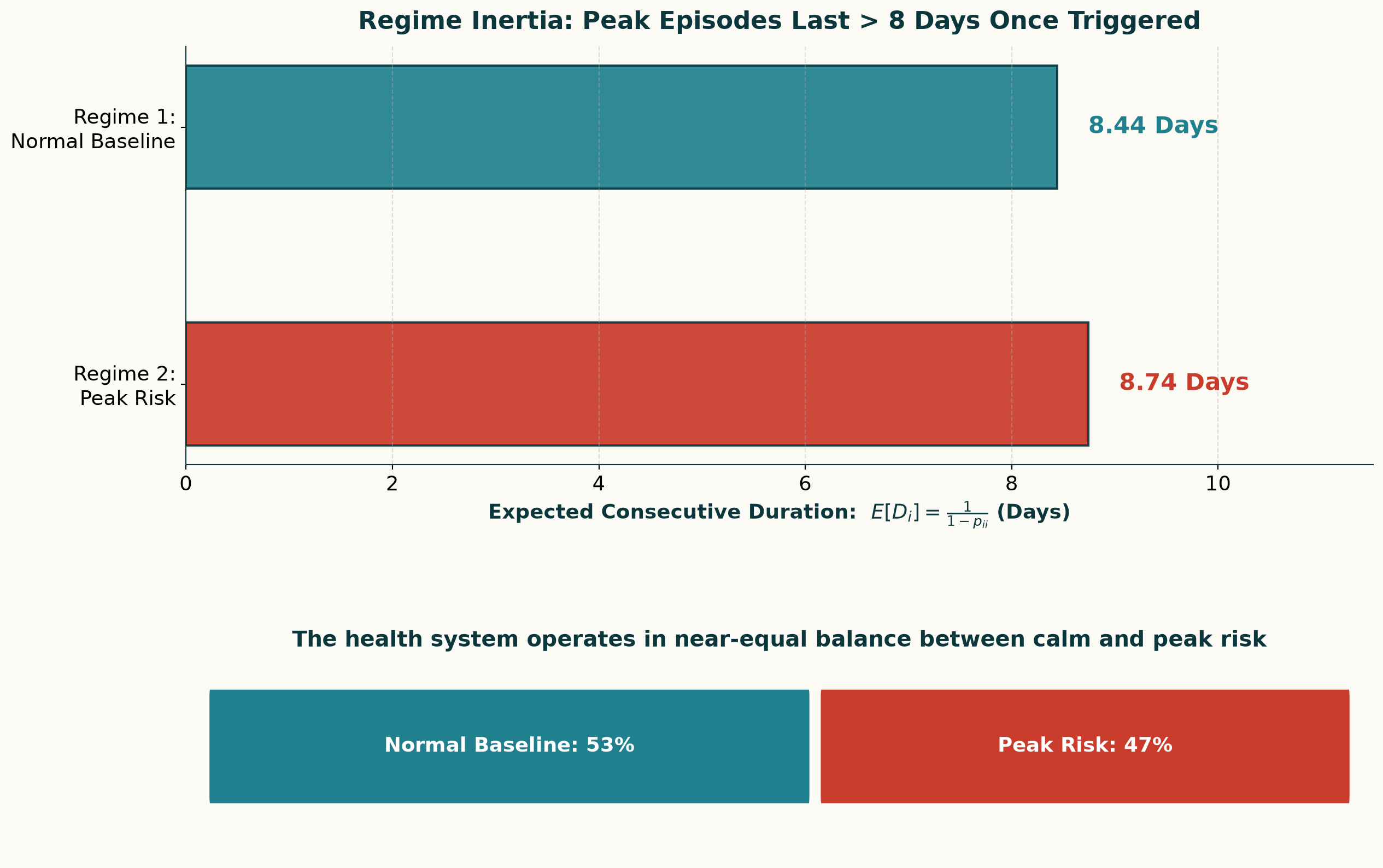
Regime Dynamics

Outline
- What Are We Forecasting?
- Model: Markov-Switching AutoRegressive Regression (MS-ARR)
- Model Results
- Data Preparation & How to Forecast Next Days in Python
- Beyond Point Forecasting
Data Preparation & Feature Engineering
| Loading ITables v2.9.1 from the internet... (need help?) |
| ⓘdate | ead | day | month | holiday | sin_365 (Annual) |
|---|---|---|---|---|---|
| 2023-03-16 | 0.34 | 3 | 3 | 0 | 0.0000 |
| 2023-03-17 | 0.48 | 4 | 3 | 0 | 0.0172 |
| 2023-03-18 | 0.57 | 5 | 3 | 0 | 0.0344 |
| 2023-03-19 | 0.50 | 6 | 3 | 0 | 0.0516 |
| 2023-03-20 | 0.83 | 0 | 3 | 0 | 0.0688 |
| 2023-03-21 | 1.12 | 1 | 3 | 0 | 0.0859 |
| 2023-03-22 | 1.10 | 2 | 3 | 0 | 0.1030 |
| 2023-03-23 | 0.98 | 3 | 3 | 0 | 0.1201 |
| 2023-03-24 | 1.51 | 4 | 3 | 0 | 0.1372 |
| 2023-03-25 | 0.54 | 5 | 3 | 0 | 0.1542 |
| (1,060 more rows not shown) | |||||
Forecasting Pipeline
import pandas as pd
ead_dff = pd.read_csv("ead_data.csv", index_col="date")
H = 5
target_var = "ead"
cat_vars = ["day", "month", "holiday"]
train_ead = ead_dff[:-H]
future_exog = ead_dff[-H:].drop(columns=target_var)
from sklearn.preprocessing import OneHotEncoder
ohe_encoder = OneHotEncoder(sparse_output=False,
                            handle_unknown='ignore',
                            drop='first')
from peshbeen.transformations import rolling_quantile
transformation_function = [rolling_quantile(
                            window_size=49,
                            quantile=0.2,
                            shift=10, min_samples=49)]
from peshbeen.models import ms_arr
ms_mod = ms_arr(n_components=2, lags=[4, 8, 10],
                target_col=target_var,
                cat_variables=cat_vars,
                categorical_encoder=ohe_encoder,
                n_iter=100,
                lag_transform=transformation_function,
                random_state=42)
ms_mod.fit(train_ead)
forecasts = ms_mod.forecast(H = H, exog=future_exog)
How Do Data Looks Like Before Passing to the Model?
| Loading ITables v2.9.1 from the internet... (need help?) |
| ⓘdate | ead | day_1 | day_2 | day_3 | day_4 | day_5 | day_6 | month_2 | month_3 | month_4 | month_5 | month_6 | month_7 | month_8 | month_9 | month_10 | month_11 | month_12 | holiday_1 | holiday_2 | holiday_3 | sin_365 (Annual) | ead_lag_4 | ead_lag_8 | ead_lag_10 | rolling_quantile_49_shift_10_q0.2 |
|---|---|---|---|---|---|---|---|---|---|---|---|---|---|---|---|---|---|---|---|---|---|---|---|---|---|---|
| 2023-05-13 | 0.53 | 0.0 | 0.0 | 0.0 | 0.0 | 1.0 | 0.0 | 0.0 | 0.0 | 0.0 | 1.0 | 0.0 | 0.0 | 0.0 | 0.0 | 0.0 | 0.0 | 0.0 | 0.0 | 0.0 | 0.0 | 0.8402 | 0.94 | 0.90 | 1.16 | 0.54 |
| 2023-05-14 | 0.61 | 0.0 | 0.0 | 0.0 | 0.0 | 0.0 | 1.0 | 0.0 | 0.0 | 0.0 | 1.0 | 0.0 | 0.0 | 0.0 | 0.0 | 0.0 | 0.0 | 0.0 | 0.0 | 0.0 | 0.0 | 0.8495 | 1.33 | 0.38 | 0.86 | 0.54 |
| 2023-05-15 | 0.85 | 0.0 | 0.0 | 0.0 | 0.0 | 0.0 | 0.0 | 0.0 | 0.0 | 0.0 | 1.0 | 0.0 | 0.0 | 0.0 | 0.0 | 0.0 | 0.0 | 0.0 | 0.0 | 0.0 | 0.0 | 0.8584 | 1.12 | 0.52 | 0.90 | 0.54 |
| 2023-05-16 | 0.64 | 1.0 | 0.0 | 0.0 | 0.0 | 0.0 | 0.0 | 0.0 | 0.0 | 0.0 | 1.0 | 0.0 | 0.0 | 0.0 | 0.0 | 0.0 | 0.0 | 0.0 | 0.0 | 0.0 | 0.0 | 0.8671 | 0.79 | 0.97 | 0.38 | 0.54 |
| 2023-05-17 | 0.46 | 0.0 | 1.0 | 0.0 | 0.0 | 0.0 | 0.0 | 0.0 | 0.0 | 0.0 | 1.0 | 0.0 | 0.0 | 0.0 | 0.0 | 0.0 | 0.0 | 0.0 | 0.0 | 0.0 | 0.0 | 0.8755 | 0.53 | 0.94 | 0.52 | 0.54 |
| 2023-05-18 | 0.39 | 0.0 | 0.0 | 1.0 | 0.0 | 0.0 | 0.0 | 0.0 | 0.0 | 0.0 | 1.0 | 0.0 | 0.0 | 0.0 | 0.0 | 0.0 | 0.0 | 0.0 | 0.0 | 0.0 | 0.0 | 0.8837 | 0.61 | 1.33 | 0.97 | 0.54 |
| 2023-05-19 | 0.30 | 0.0 | 0.0 | 0.0 | 1.0 | 0.0 | 0.0 | 0.0 | 0.0 | 0.0 | 1.0 | 0.0 | 0.0 | 0.0 | 0.0 | 0.0 | 0.0 | 0.0 | 0.0 | 0.0 | 0.0 | 0.8916 | 0.85 | 1.12 | 0.94 | 0.54 |
| 2023-05-20 | 0.31 | 0.0 | 0.0 | 0.0 | 0.0 | 1.0 | 0.0 | 0.0 | 0.0 | 0.0 | 1.0 | 0.0 | 0.0 | 0.0 | 0.0 | 0.0 | 0.0 | 0.0 | 0.0 | 0.0 | 0.0 | 0.8993 | 0.64 | 0.79 | 1.33 | 0.54 |
| 2023-05-21 | 0.33 | 0.0 | 0.0 | 0.0 | 0.0 | 0.0 | 1.0 | 0.0 | 0.0 | 0.0 | 1.0 | 0.0 | 0.0 | 0.0 | 0.0 | 0.0 | 0.0 | 0.0 | 0.0 | 0.0 | 0.0 | 0.9067 | 0.46 | 0.53 | 1.12 | 0.54 |
| 2023-05-22 | 0.36 | 0.0 | 0.0 | 0.0 | 0.0 | 0.0 | 0.0 | 0.0 | 0.0 | 0.0 | 1.0 | 0.0 | 0.0 | 0.0 | 0.0 | 0.0 | 0.0 | 0.0 | 0.0 | 0.0 | 0.0 | 0.9138 | 0.39 | 0.61 | 0.79 | 0.54 |
| (942 more rows not shown) | ||||||||||||||||||||||||||
Point Forecast Evaluation: 120-Day Out-of-Sample Horizon (example)
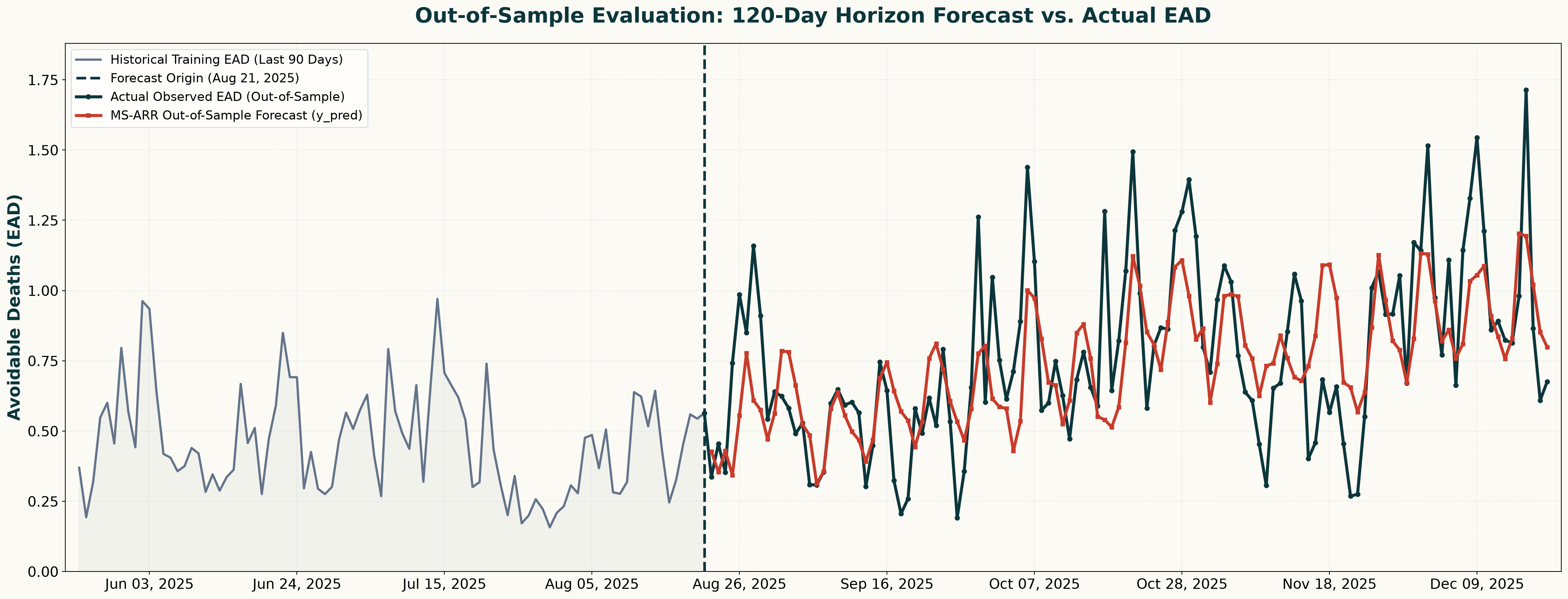
Note: Forecasts are generated once every 5 days, 24 times across 120 days.
Outline
- What Are We Forecasting?
- Model: Markov-Switching AutoRegressive Regression (MS-ARR)
- Model Results
- Data Preparation & How to Forecast Next Days in Python
- Beyond Point Forecasting
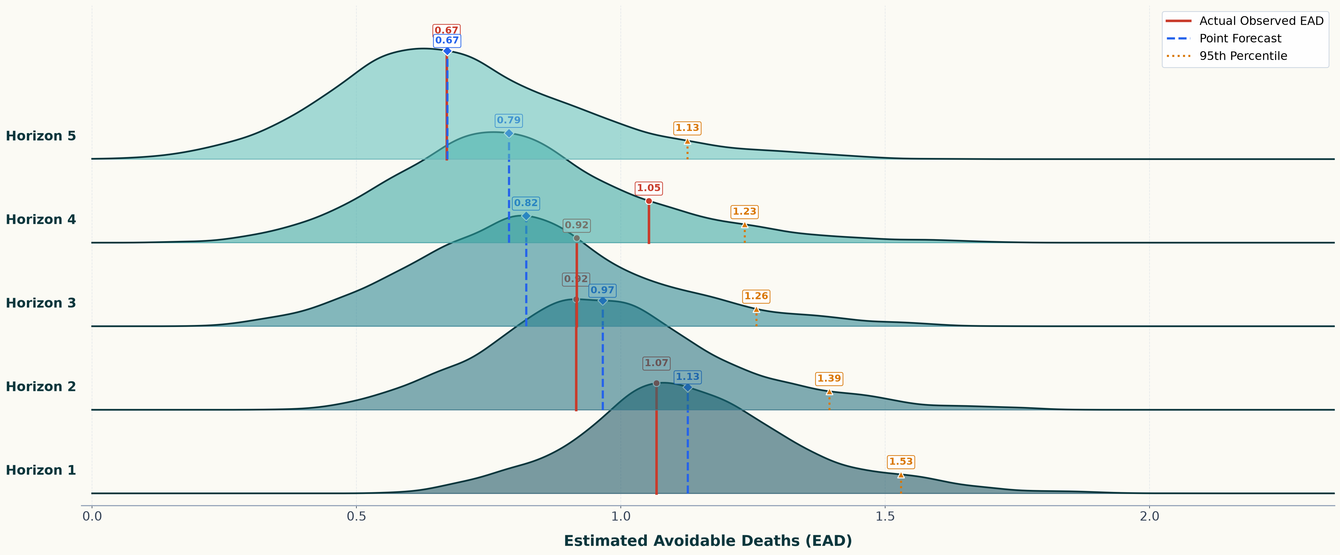
Can Point Forecasts Capture Peak Dynamics?
Forecast Distribution Across Forecast Horizons (\(h = 1 \dots 5\))
Can Calibrated Uncertainty Bounds Capture Peaks in EAD?
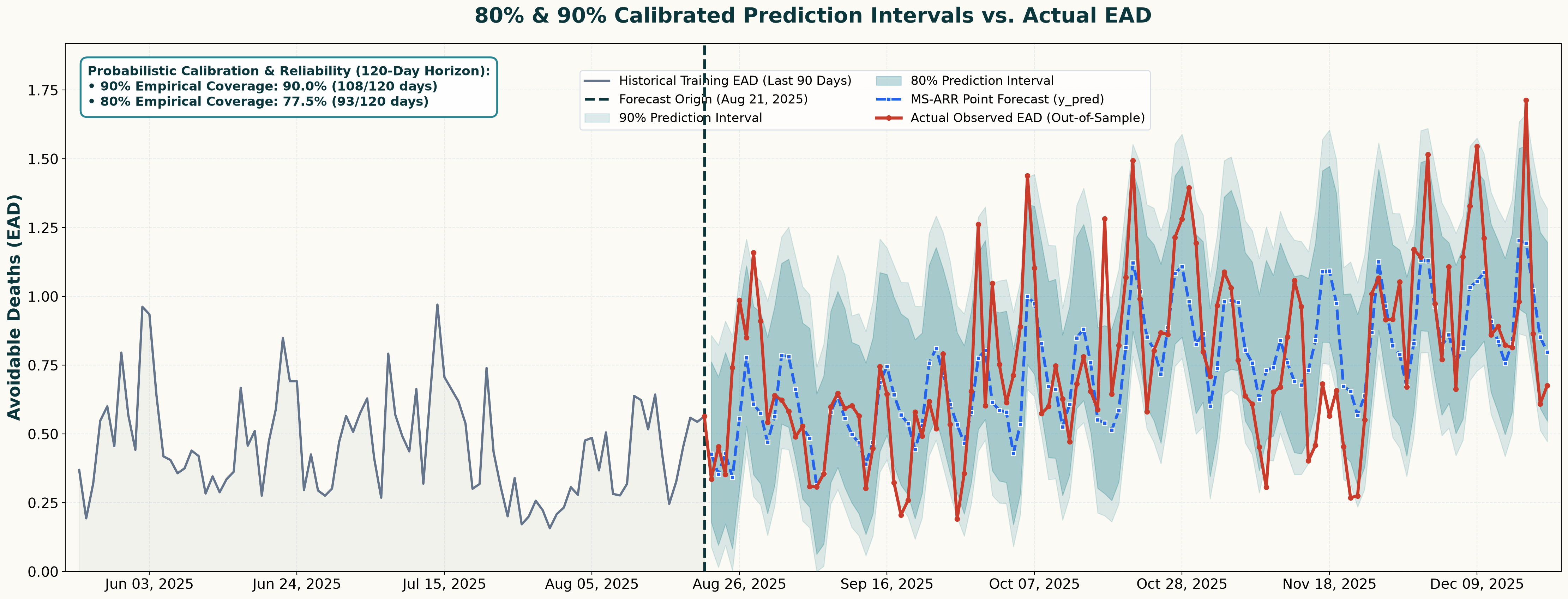
Note: Forecasts are generated once every 5 days, 24 times across 120 days.
Operationalizing Probabilistic Forecasts into Actionable Peak Signals
Any questions or thoughts? 💬