Systemic Forecasting of Hospital Patient Flow: An Interdependent Multi-Series Approach to Cross-Specialty Dynamics

6th WGSSS Postgraduate Research Conference 2026

Mustafa Aslan

Data Lab for Social Good, Cardiff Business School, Cardiff University, UK

Lead supervisor: Prof. Bahman Rostami-Tabar
Co-supervisor: Dr. Jeremy Dixon

2 November 2026 | Bangor University

Outline

Problem & Motivation
Interdependent Multi-Series Framework
Experimental Setup & Three Forecasting Approaches
Empirical Results: Point & Probabilistic Forecasting
Operational Implications & Next Steps

The Clinical & Operational Problem

Siloed Hospital Operations: Fragmented decision-making across multidisciplinary wards contributes to systemic delays, prolonged stays, and delayed discharges.
Systemic “Ripple Effects”: Admission surges in one clinical specialty act as leading indicators of downstream discharge pressure and bed blocking in others.
Patient Off-Placement: When target wards reach capacity, patients are boarded in non-specialist beds—inflating length of stay and compounding hospital gridlock.

The Scale of the Challenge

Capturing hospital-wide patient flow dynamics across 58 coupled time series

29 Clinical Specialties General Medicine, Surgery, Trauma, Cardiology, Haematology, ICU, etc.

2 Flow Types Admissions & Discharges Strongly coupled daily inflows and outflows across wards

58 Series Simultaneous Time Series 5+ years of daily NHS inpatient data (\(>109,000\) panel observations)

Central Research Questions:
1. Can exploiting interdependencies across specialties in ONE unified model improve point and probabilistic forecasts over 58 independent models?
2. Can these gains be retained using a reduced-input representation (one selected flow series per specialty)?

Conventional Baseline: 58 Independent Single-Series Models

Independent Univariate Modeling (Approach 1)

Fit 58 separate forecasting models (one per specialty and flow type).
Maintain, tune, and monitor each series in complete isolation:
- Hyperparameter tuning repeated 58 independent times (\(58 \times 75 = 4,350\) CV evaluations per model family).
Each model conditions exclusively on its own historical lags: \[ \hat{y}_{t+1}^{(i)} = f_i\left(y_t^{(i)}, y_{t-1}^{(i)}, \dots, y_{t-p}^{(i)}, \mathbf{Z}_t\right) \]

Why Siloed Forecasting Falls Short

Ignores Cross-Specialty Spillovers: Admissions and discharges are tightly coupled within and across specialties (\(r > 0.80\) in core medical/surgical wards). Univariate models are blind to upstream admission surges.
Data Fragmentation: Each model trains on only \(\sim 1,880\) daily observations rather than pooling shared seasonal and calendar structure across all \(109,000+\) hospital records.
Operational Maintenance Burden: Scaling and auditing 58 separate pipelines for point and probabilistic forecasting creates substantial technical debt.

➜ Proposed Solution: Jointly model all 58 streams via an Interdependent Multi-Series Framework

Outline

Problem & Motivation
Interdependent Multi-Series Framework
Experimental Setup & Three Forecasting Approaches
Empirical Results: Point & Probabilistic Forecasting
Operational Implications & Next Steps

Proposed Framework: Three Forecasting Architectures Compared

Evaluating full cross-series information against correlation-guided input reduction

Approach 1: Single-Series Baseline

Architecture: 58 separate models (\(f_1, \dots, f_{58}\)), tuned independently.
Lag Inputs: Own lags \(1 \dots 7\) only (\(\mathbf{7}\) lag features per model).
Cross-Series Info: None — ignores cross-specialty spillovers.

Approach 2: Multi-Series (All Lags)

Architecture: 1 unified global model \(\mathcal{M}\) predicting all 58 series at once.
Lag Inputs: Lags \(1 \dots 7\) of all 58 series (\(58 \times 7 = \mathbf{406}\) lag features).
Cross-Series Info: Full hospital-wide inflow and outflow visibility.

Approach 3: Multi-Series (Selected Lags)

Architecture: 1 unified global model \(\mathcal{M}\) with pruned cross-lags.
Lag Inputs: 1 dominant series per specialty (\(28 \times 7 = \mathbf{196}\) lags; \(-51\%\) features).
Selection Rule: Composite \(R^2\) test (\(p < 0.05, |r| \ge 0.20\)) on Adm vs. Dis.

Mathematical Formulation: Interdependent Multi-Series Model

Global Functional Mapping:
Instead of 58 disconnected functions, a single model \(\mathcal{M}\) predicts patient flow \(y_{i,t}\) for any target stream \(i \in \{1, \dots, 58\}\): \[y_{i, t} = \mathcal{M}\left( s_i, \, \mathbf{X}_{t}^{\text{cross}}, \, \mathbf{Z}_{t} \right) + \epsilon_{i, t}, \qquad i = 1, \dots, N\]
Cross-Specialty Feature Representation (\(\mathbf{X}_{t}^{\text{cross}}\)):
Concatenates \(p=7\) autoregressive lags across the active set of series \(\mathcal{S}\) (\(\mathcal{S}_{\text{full}} = 58\) series in Approach 2; \(\mathcal{S}_{\text{sel}} = 28\) dominant specialty series in Approach 3): \[\mathbf{X}_{t}^{\text{cross}} = \Big[\mathbf{y}_{t-1:t-p}^{(k)}\Big]_{k \in \mathcal{S}} \in \mathbb{R}^{|\mathcal{S}| \cdot p}\]
Pooled Empirical Risk Minimization:
Learned jointly across all \(N=58\) streams and training days via peshbeen: \[\min_{\mathcal{M}} \sum_{i=1}^{N} \sum_{t=p+1}^{T} \mathcal{L}\left( y_{i, t}, \, \mathcal{M}\left(s_i, \, \mathbf{X}_{t}^{\text{cross}}, \, \mathbf{Z}_{t}\right) \right) + \Omega(\mathcal{M})\]

Notation & Model Interface (peshbeen):

\(y_{i,t}\): Daily admissions or discharges for stream \(i\) on day \(t\)
\(s_i\): Categorical series identifier (id_col = "specialty")
\(\mathcal{S}_{\text{full}}\) vs. \(\mathcal{S}_{\text{sel}}\): 406 full lags vs. 196 selected lags
\(\mathbf{Z}_t\): Calendar (day_of_week, month), bank holidays, time trend, and capacity expansion (gm_ch)
\(\mathcal{M}(\cdot)\): Pluggable estimator in peshbeen (ml_multi_forecaster):
- LightGBM, XGBoost, CatBoost, Random Forest, Ridge

The Multi-Series Training Matrix Architecture

Time	Series ID (`id_col`)	Specialty A Lags			Specialty B Lags			Specialty C Lags			…	Exog	Target (Y) Flow
Time	Series ID (`id_col`)	lag 3	lag 2	lag 1	lag 3	lag 2	lag 1	lag 3	lag 2	lag 1	…	Exog	Target (Y) Flow
t₁	Specialty A	49	52	58	15	18	20	10	12	14	…	exog₁	65
t₂	Specialty A	52	58	65	18	20	22	12	14	16	…	exog₂	71
t₃	Specialty A	58	65	71	20	22	19	14	16	14	…	exog₃	68
↓	`id_col` switches →	← Cross-Lag Features (X) Repeat Identically Across Series →										Target switches ↓
t₁	Specialty B	49	52	58	15	18	20	10	12	14	…	exog₁	22
t₂	Specialty B	52	58	65	18	20	22	12	14	16	…	exog₂	19
t₃	Specialty B	58	65	71	20	22	19	14	16	14	…	exog₃	21
↓	`id_col` switches →	← Cross-Lag Features (X) Repeat Identically Across Series →										Target switches ↓
t₁	Specialty C	49	52	58	15	18	20	10	12	14	…	exog₁	16
t₂	Specialty C	52	58	65	18	20	22	12	14	16	…	exog₂	14
t₃	Specialty C	58	65	71	20	22	19	14	16	14	…	exog₃	15
⋮	⋮ (all 58 streams)	⋮ (cross-lags repeated identically per date across streams)										⋮

Recursive Multi-Step & Probabilistic Forecasting (\(H = 42\) Days)

Propagating cross-specialty feedback loops and joint predictive uncertainty

1. Step \(h = 1\) (Observed History)

Model ingests observed cross-series lags up to origin \(t\): \[\mathbf{X}_{t} = \left[\mathbf{y}_{t:t-6}^{(k)},\, \mathbf{Z}_{t+1}\right]_{k \in \mathcal{S}}\]
Generates 1-step ahead predictions \(\hat{\mathbf{y}}_{t+1} = \mathcal{M}(\mathbf{X}_t)\) for all 58 series simultaneously.

2. Steps \(h = 2 \dots 42\) (Recursive Roll)

Predicted flows \(\hat{\mathbf{y}}_{t+h-1}\) roll into the lag vector for step \(h\): \[\text{Lag}_1 \leftarrow \hat{\mathbf{y}}_{t+h-1}, \quad \text{Lag}_2 \leftarrow \hat{\mathbf{y}}_{t+h-2}\]
Admission surges predicted on day \(t+1\) dynamically feed into downstream specialty discharge forecasts over the 6-week horizon.

3. Joint Probabilistic Scenarios

Via multi_prob_forecasts in peshbeen, empirical residual covariance is estimated across horizons.
Generates 10,000 Monte Carlo sample paths (method="mvn") per fold, yielding full predictive distributions for every specialty and horizon \(h \in \{1, \dots, 42\}\).

Outline

Problem & Motivation
Interdependent Multi-Series Framework
Experimental Setup & Three Forecasting Approaches
Empirical Results: Point & Probabilistic Forecasting
Operational Implications & Next Steps

Experimental Design & Evaluation Protocol

NHS Inpatient Dataset & Cross-Validation Design

Dataset: Daily NHS inpatient admissions and discharges (Jan 2021 – Feb 2026; 29 specialties \(\times\) 2 flows \(= \mathbf{58}\) series).
Exogenous Covariates: Day of week, month, bank holidays, linear time index, General Medicine capacity step-change (gm_ch), plus Fourier terms & interactions for linear models.
Rolling-Origin Evaluation (SplitTimeSeries):
- 30 rolling evaluation windows, forecast horizon \(H = 42\) days (6 weeks), step size \(= 12\) days.
- Hyperparameter tuning via Optuna on the training partition (80 trials for multi-series ML; 75 trials per series for single-series).

Five Model Families & Two Evaluation Metrics

Five Diverse Learning Algorithms Evaluated Across All 3 Approaches:
1. LightGBM (lgb): Leaf-wise histogram GBDT with native categorical handling & \(L_1/L_2\) regularisation.
2. XGBoost (xgb): Depth/leaf-regularised histogram gradient boosting.
3. CatBoost (cat): Oblivious trees (symmetric splits across all nodes at a given depth).
4. Random Forest (rf): Bagged decision tree ensemble (no sequential residual boosting).
5. Ridge Regression (ridge): Linear \(L_2\)-penalised model with one-hot series & interaction encoding.
Metrics: RMSSE (Point Forecasting) and Pinball Loss across predictive quantiles (Probabilistic Forecasting).

Forecast Evaluation Metrics

Scale-independent point accuracy (RMSSE) and distributional accuracy across quantiles (Pinball Loss)

Point Forecasting: Root Mean Squared Scaled Error (RMSSE)

\[\text{RMSSE} = \sqrt{\frac{\frac{1}{H}\sum_{h=1}^{H}\left(y_{t+h} - \hat{y}_{t+h}\right)^2}{\frac{1}{T-1}\sum_{t=2}^{T}\left(y_t - y_{t-1}\right)^2}}\]

Scale-Independent Comparison: Normalises forecast errors by the in-sample one-step naïve random walk, allowing fair aggregation across high-volume (General Medicine) and low-volume specialties.
Relative Gain (%): \(\frac{\text{RMSSE}_{\text{Single}} - \text{RMSSE}_{\text{Multi}}}{\text{RMSSE}_{\text{Single}}} \times 100\).

Probabilistic Forecasting: Integrated Pinball Loss

\[L_\tau(y, \hat{q}_\tau) = \max\left(\tau(y - \hat{q}_\tau), \, (\tau - 1)(y - \hat{q}_\tau)\right)\] \[\overline{\text{PL}}(F, y) = 2 \int_0^1 L_\tau\left(y, F^{-1}(\tau)\right) d\tau\]

Full Distributional Evaluation: Assesses calibration and sharpness across all predictive quantiles \(\tau \in (0, 1)\) from 10,000 Monte Carlo trajectories across horizons \(h = 1 \dots 42\).
Lower Pinball Loss = Superior Probabilistic Quality (Skill gain \(>0\%\) indicates reduction in Pinball Loss over Single-Series).

Outline

Problem & Motivation
Interdependent Multi-Series Framework
Experimental Setup & Three Forecasting Approaches
Empirical Results: Point & Probabilistic Forecasting
Operational Implications & Next Steps

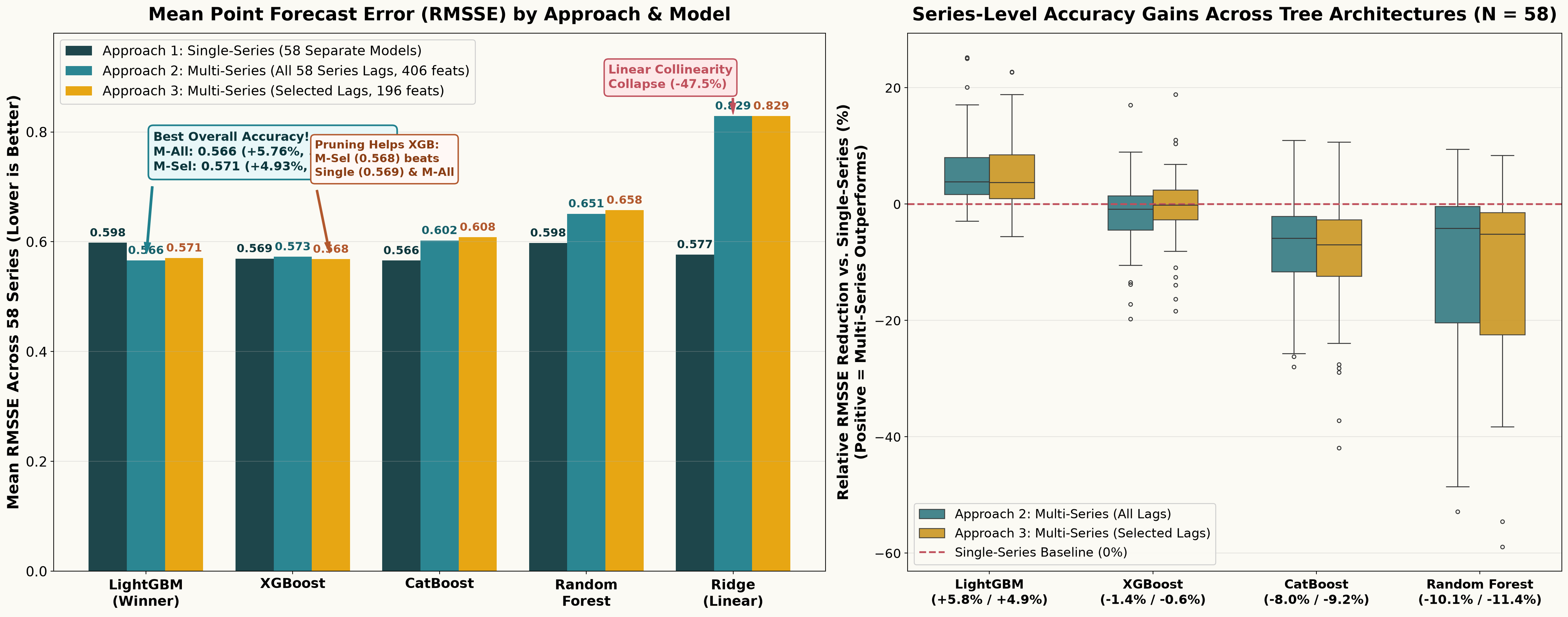
Point Forecasting Results: Comparing the Three Approaches Across Models

Why Does LightGBM Excel While Other Models Struggle?

Model architecture interaction with high-dimensional cross-series lags

LightGBM: Multi-Series Winner

Lowest Overall Error: 0.566 (All Lags) & 0.571 (Selected Lags), beating all single-series models.
Native Categorical Splits: Optimal partitioning on specialty isolates series-specific regimes.
Sparse \(L_1\) Regularisation: Filters noisy cross-lags while retaining true admission signals.

XGBoost, CatBoost & Random Forest

Input Pruning Helps XGBoost: Selected Lags (0.568) beats Single-Series (0.569) & improves 14/29 discharge series.
CatBoost (Oblivious Trees): Symmetric depth-wide splits restrict specialty-specific conditioning.
Random Forest (Bagging): Lacks sequential boosting to correct series-level biases.

Ridge: Linearity Limitation

Strong Per-Series Fit (0.577): Competitive when fitted separately with 7 own lags.
Global Collapse (0.829, \(-47.5\%\)): Forces identical cross-lag slopes across all 58 streams.
Key Takeaway: Cross-specialty spillovers are non-linear and specialty-contingent.

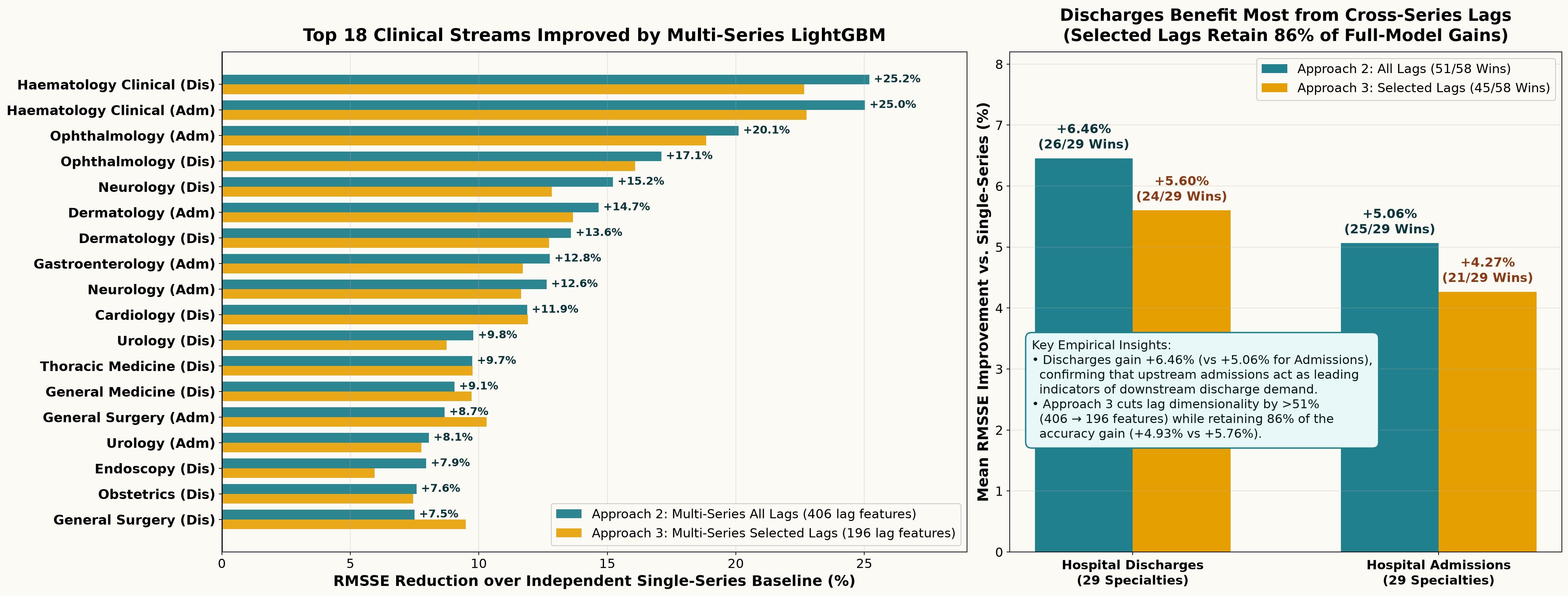
Specialty-Level Point Forecast Gains: Admissions vs. Discharges

Full-input (Approach 2) vs. Reduced-input (Approach 3) LightGBM across clinical streams

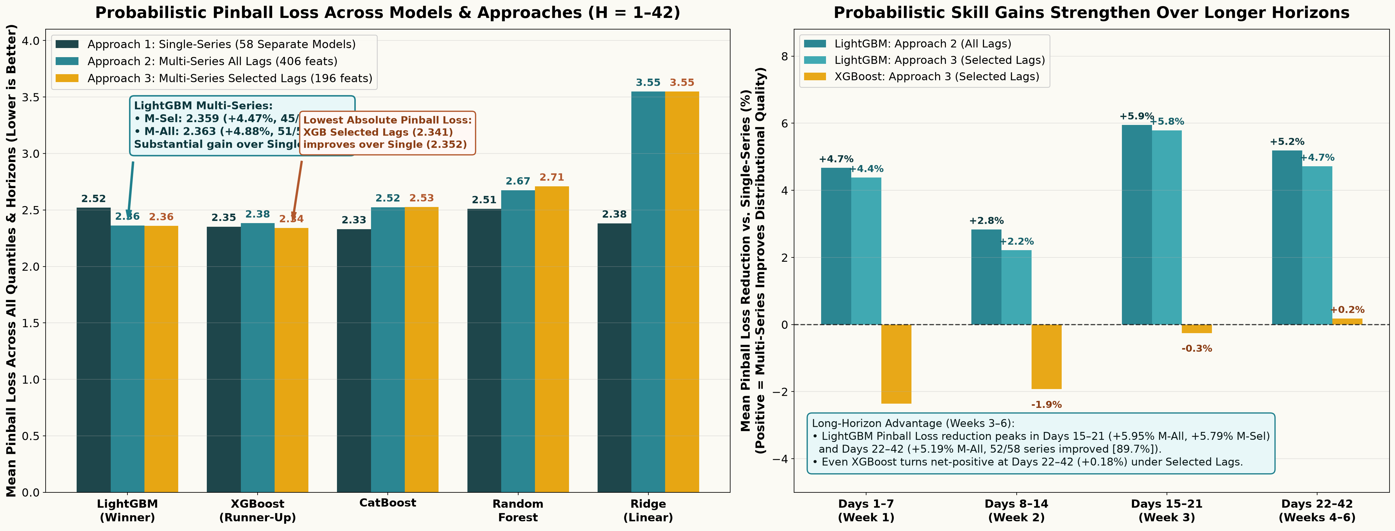
Probabilistic Forecasting Results: Pinball Loss Across Models & Horizons

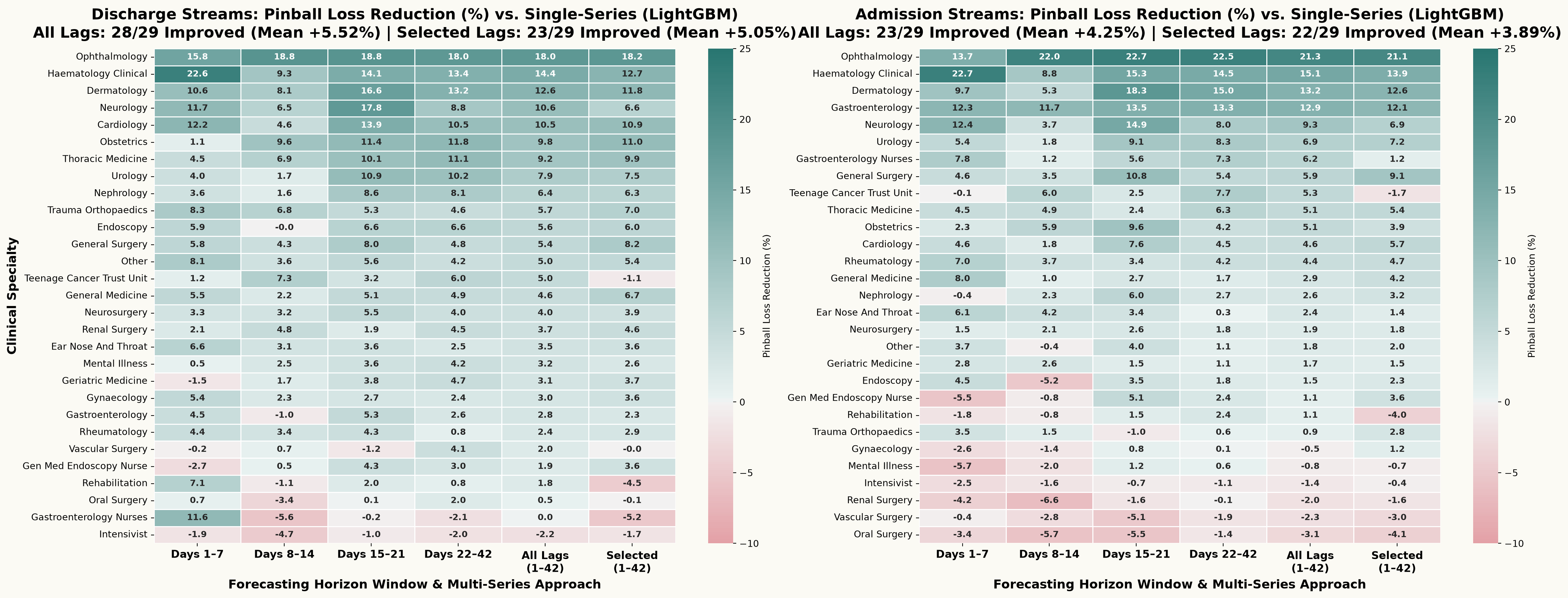
System-Wide Probabilistic Improvements Across All 58 Clinical Series

Synthesis: Comparing the Three Forecasting Approaches

Dimension	Approach 1: Single-Series	Approach 2: Multi-Series (All Lags)	Approach 3: Multi-Series (Selected Lags)	Key Takeaway
Model Count	58 separate models	1 unified model	1 unified model	98% fewer models to maintain
Lag Features	\(7\) own lags / model	\(58 \times 7 = \mathbf{406}\) lags	\(28 \times 7 = \mathbf{196}\) lags	\(-51\%\) features in Approach 3
Point Accuracy (LGB RMSSE)	\(0.598\) (Baseline)	\(0.566\) (\(+5.8\%\), \(51/58\) wins)	\(0.571\) (\(+4.9\%\), \(45/58\) wins)	Retains 86% of full-model gain
Discharges vs. Admissions	Baseline (\(0\%\))	Dis: \(+6.5\%\) (\(26/29\)) \| Adm: \(+5.1\%\)	Dis: \(+5.6\%\) (\(24/29\)) \| Adm: \(+4.3\%\)	Discharges gain most from cross-lags
Probabilistic (LGB Pinball)	\(2.520\) (Baseline)	\(2.363\) (\(+4.9\%\), \(51/58\) wins)	\(2.359\) (\(+4.5\%\), \(45/58\) wins)	Best LGB Pinball via Selected Lags
XGBoost Performance	\(0.569\) RMSSE / \(2.352\) PL	\(0.573\) RMSSE / \(2.383\) PL	\(0.568\) RMSSE / \(2.341\) PL	Lag pruning unlocks XGBoost gains

Outline

Problem & Motivation
Interdependent Multi-Series Framework
Experimental Setup & Three Forecasting Approaches
Empirical Results: Point & Probabilistic Forecasting
Operational Implications & Next Steps

Practical Implications, Limitations & Next Steps

Implications for Healthcare Operations

Proactive Discharge Planning: Cross-specialty admission signals improve discharge forecasts in 26/29 (point) and 28/29 (probabilistic) specialties, peaking in Weeks 3–6 (+5.95%).
Parsimonious Deployment (Approach 3): Selecting 1 flow series per specialty cuts lag features in half (\(406 \rightarrow 196\)) while retaining ~86–91% of accuracy gains.
Streamlined MLOps: Replaces 58 isolated models with 1 unified peshbeen pipeline.

Methodological Caveats & Next Steps

Estimator Sensitivity: Multi-series gains require learners with conditional tree splits and \(L_1\) regularisation (LightGBM); linear (Ridge) and symmetric (CatBoost) models degrade under high lag dimensionality.
From Forecasts to Bed Allocation Decisions:
- Integrate joint probabilistic trajectories into stochastic ward reservation and bed allocation optimisation to reduce patient off-placement.

Reproducible Implementation: peshbeen

Unified Forecasting Interface: Open-source Python package developed to evaluate univariate (ml_forecaster) and interdependent multi-series (ml_multi_forecaster, multi_prob_forecasts) workflows across any scikit-learn compatible estimator.

Scan for documentation

mustafaslancoto.github.io/peshbeen

Any questions or thoughts? 💬