Automatic Encoding for Categorical Variables

To encode calendar features as categorical variables, we can use any suitable encoding method from the sklearn.preprocessing module, such as OneHotEncoder, TargetEncoder, or OrdinalEncoder.

In three examples, we will use OneHotEncoder to encode the categorical variables in our dataset. This method creates new binary columns for each category in the original variable.

from sklearn.preprocessing import OneHotEncoder
import numpy as np
import pandas as pd
from peshbeen.models import ml_forecaster
from lightgbm import LGBMRegressor
from xgboost import XGBRegressor

date_range = pd.date_range(start='2020-01-01', periods=720, freq='D')
# create a non-stationary arbitrary flower sales data with an upward trend, weekly seasonality, and yearly seasonality
np.random.seed(42)
data = 30 + 0.07 * np.arange(720) + 10 * np.sin(2 * np.pi * date_range.dayofyear / 7) + 10 * np.sin(2 * np.pi * date_range.dayofyear / 365) + np.random.normal(0, 5, 720)

sales_data = pd.DataFrame(data, index=date_range, columns=['sales'])
sales_data["week_day"] = sales_data.index.dayofweek
sales_data["month"] = sales_data.index.month
cat_vars = ["week_day", "month"]
train = sales_data.iloc[:-30]
test = sales_data.iloc[-30:]

# Example of using OneHotEncoder for XGBoost
ohe = OneHotEncoder(sparse_output=False, handle_unknown="ignore", drop="first")

xgb = ml_forecaster(target_col="sales", model=XGBRegressor(n_estimators=100, random_state=42),
                    lags = 6,
                    cat_variables=cat_vars, categorical_encoder=ohe)
xgb.fit(train)
xgb_forecasts = xgb.forecast(30, exog=test[cat_vars])

# How the transformed features look like for XGBoost
xgb.X.head()

	week_day_1	week_day_2	week_day_3	week_day_4	week_day_5	week_day_6	month_2	month_3	month_4	month_5	...	month_9	month_10	month_11	month_12	sales_lag_1	sales_lag_2	sales_lag_3	sales_lag_4	sales_lag_5	sales_lag_6
2020-01-07	1.0	0.0	0.0	0.0	0.0	0.0	0.0	0.0	0.0	0.0	...	0.0	0.0	0.0	0.0	22.392017	20.219602	34.174336	38.233477	39.472174	40.474019
2020-01-08	0.0	1.0	0.0	0.0	0.0	0.0	0.0	0.0	0.0	0.0	...	0.0	0.0	0.0	0.0	39.518145	22.392017	20.219602	34.174336	38.233477	39.472174
2020-01-09	0.0	0.0	1.0	0.0	0.0	0.0	0.0	0.0	0.0	0.0	...	0.0	0.0	0.0	0.0	43.518276	39.518145	22.392017	20.219602	34.174336	38.233477
2020-01-10	0.0	0.0	0.0	1.0	0.0	0.0	0.0	0.0	0.0	0.0	...	0.0	0.0	0.0	0.0	39.504995	43.518276	39.518145	22.392017	20.219602	34.174336
2020-01-11	0.0	0.0	0.0	0.0	1.0	0.0	0.0	0.0	0.0	0.0	...	0.0	0.0	0.0	0.0	39.394569	39.504995	43.518276	39.518145	22.392017	20.219602

5 rows × 23 columns

## Example of using TargetEncoder for LightGBM
from sklearn.preprocessing import TargetEncoder
te = TargetEncoder(cv=5)
lgb = ml_forecaster(target_col="sales", model=LGBMRegressor(n_estimators=100, random_state=42, verbose=-1),
                    lags = 6,
                    cat_variables=cat_vars, categorical_encoder=te)
lgb.fit(train)
lgb_forecasts = lgb.forecast(30, exog=test[cat_vars])

# How the transformed features look like for LightGBM
lgb.X.head()

	week_day	month	sales_lag_1	sales_lag_2	sales_lag_3	sales_lag_4	sales_lag_5	sales_lag_6
2020-01-07	50.118039	46.945004	22.392017	20.219602	34.174336	38.233477	39.472174	40.474019
2020-01-08	55.195593	47.235865	39.518145	22.392017	20.219602	34.174336	38.233477	39.472174
2020-01-09	59.591927	46.210753	43.518276	39.518145	22.392017	20.219602	34.174336	38.233477
2020-01-10	59.436795	46.478067	39.504995	43.518276	39.518145	22.392017	20.219602	34.174336
2020-01-11	57.761881	49.035528	39.394569	39.504995	43.518276	39.518145	22.392017	20.219602

Automatic Transformations for Rolling Window Features

peshbeen supports user-specified rolling window features — such as rolling means and standard deviations — which can be particularly useful for ML regressors as they capture recent dynamics in the series. Beyond feature engineering, peshbeen can automatically apply a Box-Cox transformation to the target variable when the data exhibits heteroscedasticity, stabilising variance before model fitting and improving forecast reliability.

import matplotlib.pyplot as plt
from peshbeen.transformations import rolling_mean, rolling_quantile, rolling_std, expanding_mean
from peshbeen.models import ml_forecaster
from sklearn.linear_model import LinearRegression

transformations = [rolling_std(window_size=30, shift=1), rolling_mean(window_size=30, shift=7),
                   rolling_quantile(window_size=30, shift=1, quantile=0.25),
                   rolling_quantile(window_size=30, shift=1, quantile=0.75), expanding_mean(shift=1)]
linear_model = ml_forecaster(model=LinearRegression(),
              target_col='sales', lags = 7, box_cox=0.5,
              lag_transform=transformations, cat_variables=cat_vars, categorical_encoder=ohe)
linear_model.fit(train)
# linear_model.data_prep(train)
forecasts = linear_model.forecast(H=30, exog=test[cat_vars])

# plot the forecast and the actual values
plt.figure(figsize=(12, 6))
plt.plot(train.index[-120:], train['sales'][-120:], label='Train')
plt.plot(test.index, test['sales'], label='Test')
plt.plot(test.index, forecasts, label='Linear Regression Forecast')
plt.title('Linear Regression Forecast')
plt.xlabel('Date')
plt.ylabel('Sales')
plt.legend()
plt.show()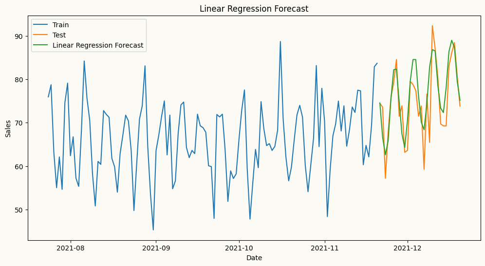

# How the transformed features look like for Linear Regression
linear_model.X.head()

	week_day_1	week_day_2	week_day_3	week_day_4	week_day_5	week_day_6	month_2	month_3	month_4	month_5	...	sales_lag_3	sales_lag_4	sales_lag_5	sales_lag_6	sales_lag_7	rolling_std_30_shift_1	rolling_mean_30_shift_7	rolling_quantile_30_shift_1_q0.25	rolling_quantile_30_shift_1_q0.75	expanding_mean_shift_1
2020-01-08	0.0	1.0	0.0	0.0	0.0	0.0	0.0	0.0	0.0	0.0	...	6.993242	9.691764	10.366645	10.565377	10.723839	1.581041	10.723839	8.577902	10.569034	9.482514
2020-01-09	0.0	0.0	1.0	0.0	0.0	0.0	0.0	0.0	0.0	0.0	...	7.464041	6.993242	9.691764	10.366645	10.565377	1.583857	10.644608	9.134833	10.610479	9.696410
2020-01-10	0.0	0.0	0.0	1.0	0.0	0.0	0.0	0.0	0.0	0.0	...	10.572692	7.464041	6.993242	9.691764	10.366645	1.509947	10.551954	9.691764	10.572692	9.793542
2020-01-11	0.0	0.0	0.0	0.0	1.0	0.0	0.0	0.0	0.0	0.0	...	11.193677	10.572692	7.464041	6.993242	9.691764	1.443708	10.336906	9.860484	10.572169	9.869489
2020-01-12	0.0	0.0	0.0	0.0	0.0	1.0	0.0	0.0	0.0	0.0	...	10.570600	11.193677	10.572692	7.464041	6.993242	1.460908	9.668173	8.937674	10.571646	9.716225

5 rows × 29 columns

Fourier Terms for Seasonal Patterns

For series with strong seasonal patterns, peshbeen can automatically generate Fourier terms as a DataFrame indexed to match the original series — making them ready to merge as exogenous variables in a single line. Calendar features such as month or day of week can be added directly to the same DataFrame, and peshbeen will automatically encode them as categorical variables. This covers a wide range of calendar effects, from weekend sales spikes to holiday demand shifts.

from peshbeen.transformations import fourier_terms
# create fourier terms for yearly seasonality with period 365 and number of terms 2 to be used as exogenous variables in the model
sales_exog = sales_data.copy() # create a copy of the original data to store the fourier terms

sales_exog.drop(columns=["month"], inplace=True) # drop month column because we will use fourier terms to capture the yearly seasonality instead of using month as a categorical variable
fourier_trms = fourier_terms(index=sales_exog.index, period=365, num_terms=2)
sales_exog = sales_exog.merge(fourier_trms, left_index=True, right_index=True) # merge the fourier terms with the original data to be used as exogenous variables in the model
sales_exog.head()

	sales	week_day	sin_1_365	sin_2_365	cos_1_365	cos_2_365
2020-01-01	40.474019	2	0.000000	0.000000	1.000000	1.000000
2020-01-02	39.472174	3	0.017213	0.034422	0.999852	0.999407
2020-01-03	38.233477	4	0.034422	0.068802	0.999407	0.997630
2020-01-04	34.174336	5	0.051620	0.103102	0.998667	0.994671
2020-01-05	20.219602	6	0.068802	0.137279	0.997630	0.990532

# split the data into train and test
from sklearn.linear_model import Lasso
train_exog = sales_exog.iloc[:-30]
test_exog = sales_exog.iloc[-30:].drop(columns=['sales']) # drop the target column from the exogenous variables for the test set
# ml forecast using Linear Regression with fourier terms as exogenous variables
lr_model = ml_forecaster(model=Lasso(alpha=0.1),
              target_col='sales', lags = 7, lag_transform=transformations,
              cat_variables=["week_day"], categorical_encoder=ohe)
lr_model.fit(train_exog)
lr_forecast = lr_model.forecast(H=30, exog=test_exog)
# plot the forecast and the actual values
plt.figure(figsize=(12, 6))
plt.plot(train.index[-120:], train['sales'][-120:], label='Train')
plt.plot(test.index, test['sales'], label='Test')
plt.plot(test.index, lr_forecast, label='Linear Regression Forecast with Fourier Terms')
plt.title('Linear Regression Forecast with Fourier Terms')
plt.xlabel('Date')
plt.ylabel('Sales')
plt.legend()
plt.show()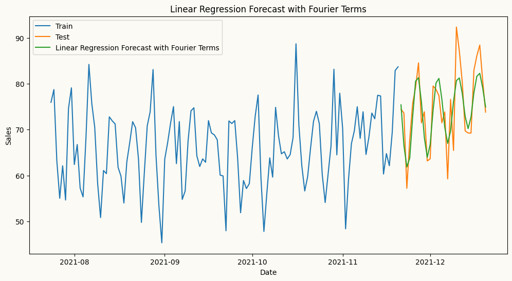

A wider set of rolling and expanding transforms

Besides rolling_mean, rolling_std, and rolling_quantile, peshbeen also exposes rolling_min and rolling_max (window extremes), and the expanding-window family expanding_mean, expanding_std, and expanding_quantile. Each takes a shift (how far back the window ends, to avoid leakage); the rolling classes take a window_size, and the quantile classes take a quantile. You mix and match them in the lag_transform list exactly like the transforms above.

from peshbeen.transformations import (rolling_min, rolling_max,
                                      expanding_std, expanding_quantile)

extra_transforms = [
    rolling_min(window_size=14, shift=1),
    rolling_max(window_size=14, shift=1),
    expanding_std(shift=1),
    expanding_quantile(shift=1, quantile=0.9),
]

extra_model = ml_forecaster(model=LinearRegression(),
              target_col='sales', lags=7,
              lag_transform=extra_transforms,
              cat_variables=cat_vars, categorical_encoder=ohe)
extra_model.fit(train)
extra_forecasts = extra_model.forecast(H=30, exog=test[cat_vars])

# the generated feature columns now include the new rolling/expanding stats
extra_model.X.head()

	week_day_1	week_day_2	week_day_3	week_day_4	week_day_5	week_day_6	month_2	month_3	month_4	month_5	...	sales_lag_2	sales_lag_3	sales_lag_4	sales_lag_5	sales_lag_6	sales_lag_7	rolling_min_14_shift_1	rolling_max_14_shift_1	expanding_std_shift_1	expanding_quantile_shift_1_q0.9
2020-01-08	0.0	1.0	0.0	0.0	0.0	0.0	0.0	0.0	0.0	0.0	...	22.392017	20.219602	34.174336	38.233477	39.472174	40.474019	20.219602	40.474019	8.593977	39.900494
2020-01-09	0.0	0.0	1.0	0.0	0.0	0.0	0.0	0.0	0.0	0.0	...	39.518145	22.392017	20.219602	34.174336	38.233477	39.472174	20.219602	43.518276	8.709596	41.387296
2020-01-10	0.0	0.0	0.0	1.0	0.0	0.0	0.0	0.0	0.0	0.0	...	43.518276	39.518145	22.392017	20.219602	34.174336	38.233477	20.219602	43.518276	8.299812	41.082871
2020-01-11	0.0	0.0	0.0	0.0	1.0	0.0	0.0	0.0	0.0	0.0	...	39.504995	43.518276	39.518145	22.392017	20.219602	34.174336	20.219602	43.518276	7.932650	40.778445
2020-01-12	0.0	0.0	0.0	0.0	0.0	1.0	0.0	0.0	0.0	0.0	...	39.394569	39.504995	43.518276	39.518145	22.392017	20.219602	20.219602	43.518276	8.080891	40.474019

5 rows × 28 columns

Per-series transforms in multivariate models. In the multivariate forecasters (var, ml_mv_forecaster, ms_var), lag_transform accepts a dictionary keyed by target column, so each series can carry its own set of rolling/expanding features — e.g. lag_transform={'sales': [rolling_mean(window_size=7, shift=1)], 'marketing': [rolling_std(window_size=14, shift=1)]}. This mirrors the per-series lags dictionary shown in the model-zoo guide.

Box-Cox bias adjustment. When you set box_cox=True (or a numeric lambda) on any forecaster, pass box_cox_biasadj=True to apply the bias correction when the prediction is back-transformed to the original scale — this corrects the systematic downward bias of a naive inverse Box-Cox and yields mean (rather than median) forecasts.