from peshbeen.datasets import load_wales_admissions # addmissions to E&A hospitals in Wales
from peshbeen.models import ml_forecaster
from peshbeen.transformations import rolling_mean, rolling_std, expanding_mean
from xgboost import XGBRegressor
wales_admissions = load_wales_admissions()
wales_admissions["day_of_week"] = wales_admissions.index.dayofweek # add day of week as a feature
wales_admissions["month"] = wales_admissions.index.month # add month as a feature to capture seasonality
wales_admissions["day_of_month"] = wales_admissions.index.day # add day of month as a feature to capture seasonality
# split the data into train and test sets
train = wales_admissions[:-30]
test = wales_admissions[-30:]
cat_variables = ["day_of_week", "month", "day_of_month"]
from sklearn.preprocessing import OneHotEncoder
ohe = OneHotEncoder(drop='first', sparse_output=False, handle_unknown="ignore")
transforms = [rolling_mean(window_size= 28, shift=7), rolling_std(window_size=28), expanding_mean()]
# import linear regression from sklearn
from sklearn.linear_model import LinearRegression
ml_linear = ml_forecaster(model=XGBRegressor(),
target_col='admissions', lags = 6,
cat_variables=cat_variables, categorical_encoder=ohe,
lag_transform=transforms)
ml_linear.fit(train)
forecasts = ml_linear.forecast(H=30, exog=test[cat_variables])![]()


![]()
![]()
![]()
![]()


One forecasting workflow. Many models. From classical statistics to machine learning, regime-switching, and probabilistic scenarios — all behind the same
.fit(df)/.forecast(H)interface.
Peshbeen is a Python forecasting library built around a single idea: the forecasting workflow should be the same regardless of the model. The name draws from Kurdish — pesh (“front”) and been (“to see”) — combining to mean foresight.
Most forecasting libraries make you pick a lane: a classical-statistics toolkit, an ML-regressor framework, or a deep-learning stack — each with its own API, its own feature-engineering conventions, and its own way of handling trends and uncertainty. Peshbeen instead puts an unusually wide range of models behind one consistent interface, and bakes in the parts of a real forecasting workflow — feature engineering, trend handling, probabilistic scenarios, tuning, and model comparison — so switching models is a one-line change, not a rewrite.
It spans naive baselines, ETS, ARIMA, Vector Autoregression (VAR), scikit-learn regressors and gradient-boosted trees (XGBoost, LightGBM, CatBoost), TabPFN tabular foundation models, Generalized Linear Models (GLM) for count data, Markov-switching regime models (MS-ARR and MS-VAR), and a built-in weighted ensemble (pesh) — for univariate and multivariate series.
Why peshbeen?
Peshbeen is designed for the messy middle of real-world forecasting — the projects where you need to try several very different model families, account for structural breaks and regime changes, model counts as well as continuous demand, and produce uncertainty you can actually feed into a decision. Its advantages:
🔁 Switch models without rewriting your code. A naive baseline, an ARIMA, a LightGBM regressor, a VAR, and a Markov-switching model all share the same
.fit/.forecast/.cross_validateAPI. Comparing them fairly is a one-line change, not a new pipeline.🌀 Regime-switching, built in. First-class Markov-switching autoregressive (
ms_arr) and VAR (ms_var) models capture regime changes — crisis vs. baseline demand, pre/post-intervention — that ARIMA and standard ML models smooth over. These sit behind the same interface as every other model.📈 A unified trend / stationarity pipeline across all model families. Differencing, a global linear trend, a local ETS trend, or piecewise-linear detrending with explicit change points is a single model argument — and it behaves identically whether you’re running ARIMA, a GLM, gradient boosting, or a regime-switching model. No rebuilding a transformer pipeline per model.
🔗 Multivariate forecasting with per-series control.
var,ml_mv_forecaster, andms_varaccept a dictionary of lags (and transformations) per target series, so each series can carry its own temporal structure while you still model their interdependencies.🎲 Probabilistic scenarios, not just intervals. Generate full sample paths for any model via residual calibration — empirical bootstrap, KDE, or a correlated (block) bootstrap that preserves dependence across horizons — ready to drop into capacity-planning or queueing simulations. Conformal prediction is available when you only need calibrated intervals.
🔢 Counts as a first-class case. A statsmodels-backed GLM with a proper
family(e.g.sm.families.Poisson(), Gamma) handles count data — admissions, calls, demand — directly, with AIC/BIC/HQC reported.🧰 Batteries included. Automatic lag and rolling/expanding feature generation, Box-Cox stabilisation, Hyperopt/Optuna tuning, forward/backward feature selection, a built-in metric-optimised ensemble (
pesh), and ready-to-use datasets (including real healthcare operations series).
A note on what powers it. Peshbeen stands on proven foundations rather than reinventing them: its ARIMA is built on StatsForecast and its ETS/GLM on statsmodels. The value peshbeen adds is the unified workflow around them — plus genuinely original pieces like the Markov-switching models, the per-series multivariate specification, the shared change-point-aware detrending, and the
peshensemble.
Key Features
The advantages above, in detail:
Unified API: Train any model using a simple
.fit(df)and.forecast(H)workflow, eliminating the need for manual feature/target splitting.Model Agnostic: Supports a wide range of forecasting models behind one interface — naive baselines, ETS, ARIMA, Vector Autoregressions, scikit-learn regressors, gradient-boosted trees (XGBoost, LightGBM, CatBoost), TabPFN foundation models, Generalized Linear Models (GLM) for count data, and Markov-switching regime models (MS-ARR, MS-VAR).
Automatic Feature Engineering: User can specify the key following parameters to automatically generate features:
lags: List of lag periods to create lag features.rolling_windows: List of window sizes for rolling statistics to create rolling features (e.g., rolling mean, rolling std, rolling quantiles).trend removal: Option to automatically difference the data or de-trend it using global trend, local trend, or piecewise linear trend. For piecewise linear trend, the user can specify the indexes of the breakpoints. For local trend, the user can pass ETS parameters to fit a local ETS model and use its fitted values as the local trend.boxcox: Option to apply Box-Cox transformation to target variable to stabilize variance.
Multivariate Forecasting: Supports forecasting with multiple target variables and exogenous regressors, making it suitable for multivariate forecasting tasks where relationships between variables can be leveraged for improved accuracy.
Probabilistic Forecasting: Enables probabilistic forecasting through a simple two-step workflow. First, call
calibratewith a held-out portion (calibration data) of your dataset — peshbeen uses the residuals at each horizon to fit the uncertainty model. Then callsampleto generate forecast scenarios and prediction intervals, giving you a full picture of forecast uncertainty for risk assessment and decision-making.Four methods are implemented for generating probabilistic forecasts:
Empirical bootstrap: Resamples from the empirical distribution of the residuals and adds the resampled residuals to the point forecasts, building a distribution of possible future values (
method="empirical").Kernel Density Estimation (KDE): Fits a smooth probability density to the residuals and samples from it, which can capture non-normal or heteroscedastic residual structure better than plain resampling (
method="kde").Correlated (block) bootstrap: Resamples entire rows of residuals (all horizons together), preserving the temporal dependencies and correlations between forecast errors at different horizons for more realistic scenarios (
method="correlated").Conformal prediction: Calculates nonconformity scores from the residuals on a calibration set and uses them to construct prediction intervals. This method produces intervals only (no scenario sample paths), and is accessed via
calibrate()+conformal_quantiles().
Hyperparameter Tuning & Feature Selection: Built-in hyperparameter tuning with Hyperopt and Optuna, plus forward/backward feature selection, so you can optimise both model configuration and the feature set with minimal effort.
Built-in Ensemble (
pesh): Combine any set of fitted models with equal weights, user-defined weights, or weights optimised to minimise the metric you care about via cross-validation.Evaluation Metrics: A metrics module covering MAE, MSE, RMSE, MAPE, SMAPE, WMAPE and the scaled metrics MASE, RMSSE and SRMSE for fair model comparison.
When to reach for peshbeen
Peshbeen is the right tool when you want to compare statistical, ML, and regime-switching models with the same code, when you suspect regime changes or structural breaks, when you’re forecasting counts, when your multivariate series need different lag structures, or when you need forecast scenarios for downstream simulation rather than just a point and an interval.
If your problem is dominated by deep-learning / foundation models, or by fitting thousands of series at maximum speed, mature specialised libraries (Darts, sktime, Nixtla) may serve you better — and peshbeen happily wraps the same proven engines where it makes sense. Peshbeen’s focus is coherence across a wide model span and coverage of an underserved middle, not out-scaling any single category.
Installation
Installation requires Python 3.10 or higher.
Core install
Installs only the essential dependencies (numpy, pandas, scipy, scikit-learn, statsmodels):
pip install peshbeenOptional dependencies
Install only what you need:
pip install peshbeen[ml]        # XGBoost, LightGBM, CatBoost, Cubist
pip install peshbeen[tuning]    # Hyperopt, Optuna
pip install peshbeen[all]       # Everything above
Quick Start Example
## Plot the historical data
import matplotlib.pyplot as plt
wales_admissions["admissions"].plot(figsize=(10, 6), label='Admissions')
plt.title("Daily Admissions to E&A Hospitals in Wales")
plt.xlabel("Date")
plt.ylabel("Number of Admissions")
plt.show()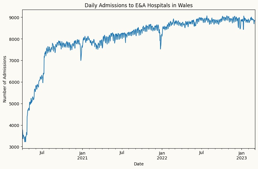
# plot the forecast against the actual values
plt.figure(figsize=(10, 6))
plt.plot(train.index[-90:], train['admissions'][-90:], label='Train')
plt.plot(test.index, test['admissions'], label='Test')
plt.plot(test.index, forecasts, label='Forecast')
plt.legend()
plt.show()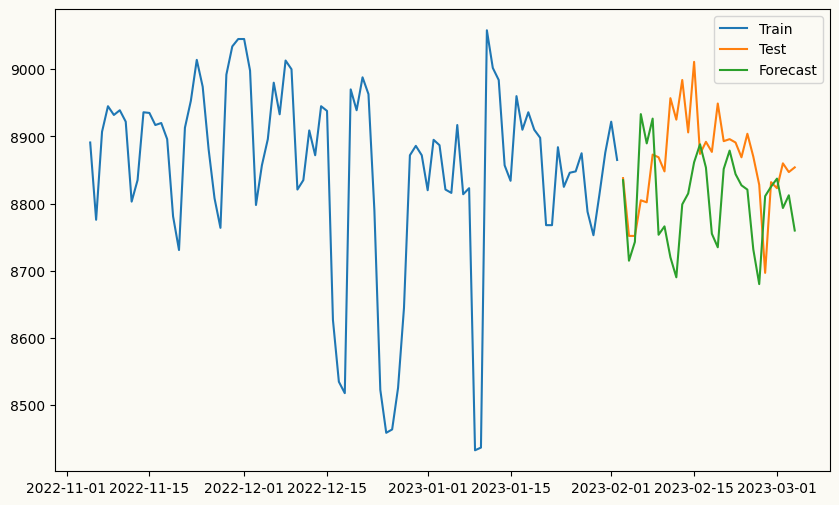
Acknowledgements
Sincere thanks to the Data Lab for Social Good research group at Cardiff University, UK, and its Director, Prof. Bahman Rostami-Tabar, for their support and encouragement during the development of this package.

Developers
- Mustafa Aslan, PhD Researcher in Data Science and Operations Research in Healthcare Operations at Cardiff University.
Contributions, issues, and feature requests are welcome on the GitHub repository.
References & Gratitude
Peshbeen would not exist without the valuable work of the respective researchers and practitioners. The following references are the foundation of this package — they shaped its methods, its design, and the way it thinks about forecasting. I am deeply grateful to their authors for making such clear, generous, and freely available scholarship.
Forecasting foundations
Hyndman, R.J., & Athanasopoulos, G. (2021). Forecasting: Principles and Practice (3rd ed.). OTexts.
Kolassa, S., Rostami-Tabar, B., & Siemsen, E. (2023). Demand Forecasting for Executives and Professionals. Chapman & Hall/CRC. (free online edition)
Hamilton, J. D. (1994). Time Series Analysis. Princeton University Press. Time Series Analysis
Jurafsky, D., & Martin, J.H. (2024). Hidden Markov Models (Appendix A). In Speech and Language Processing (3rd ed. draft)